Last Updated on 03/03/2026 by Eran Feit
Introduction
Welcome to our comprehensive Dinosaur Image Classification Tutorial!
Let’s learn a simple way for Dinosaur lower Classifications 🦕
Check out our tutorial here : https://www.youtube.com/watch?v=ZhTGcw0C3Dk
Link for the full code here : https://eranfeit.lemonsqueezy.com/buy/f4d35093-1b80-4643-821c-45b407b0b348 or here : https://ko-fi.com/s/a902042be9
This hands-on tutorial walks you through building a Convolutional Neural Network (CNN) to classify 5 dinosaur categories from images.
We’ll cover dataset prep, model architecture, training, and evaluation — and finish with tips to improve accuracy.
We’ll learn how use Convolutional Neural Network (CNN) to classify 5 dinosaur categories , based on 200 images :
- Data Preparation: We’ll begin by downloading a curated dataset of dinosaur images, neatly categorized into five distinct classes. You’ll learn how to load and preprocess the data using Python, OpenCV, and Numpy, ensuring it’s perfectly ready for training.
- CNN Architecture: Unravel the secrets of Convolutional Neural Networks (CNNs) as we dive into their structure and discuss the different layers—convolutional, pooling, and fully connected. Learn how these layers work together to extract meaningful features from images.
- Model Training : Using Tensorflow and Keras , we will define and train our custom CNN model. We’ll configure the loss function, optimizer, and evaluation metrics to achieve optimal performance during training.
- Evaluation Metrics: We’ll evaluate our trained model using various metrics like accuracy and confusion matrix to measure its efficiency and robustness.
- Predicting New Images: Finally , We put our pre-trained model to the test! We’ll showcase how to use the model to make predictions on fresh, unseen dinosaur images, and witness the magic of AI in action.
You can find more tutorials, and join my newsletter here : https://eranfeit.net/
Prerequisites
- Python 3.9+
tensorflow,keras,opencv-python,numpy,matplotlib- A folder layout like:
Simple Dinosaur Dataset/ ├─ ClassA/ ├─ ClassB/ ├─ ... Want the exact dataset so your results match mine?
If you want to reproduce the same training flow and compare your results to mine, I can share the dataset structure and what I used in this tutorial. Send me an email and mention the name of the tutorial / dataset , so I know what you’re requesting.
Here is the code for the project :
1) Setup & Data Loading
import os import numpy as np import cv2 from keras.preprocessing.image import ImageDataGenerator # Path to your dataset (change to your path) path = r"E:/Data-sets/Simple Dinosaur Dataset" # Derive classes from folder names categories = sorted(os.listdir(path)) num_classes = len(categories) print("Classes:", categories, "| #:", num_classes) # Parameters BATCH_SIZE = 32 IMG_SIZE = (224, 224) # Train/valid generators with light augmentation datagen = ImageDataGenerator( rescale=1./255, validation_split=0.2, horizontal_flip=True ) train_ds = datagen.flow_from_directory( path, target_size=IMG_SIZE, batch_size=BATCH_SIZE, subset="training", class_mode="categorical", shuffle=True ) valid_ds = datagen.flow_from_directory( path, target_size=IMG_SIZE, batch_size=BATCH_SIZE, subset="validation", class_mode="categorical", shuffle=True ) Link for the full code : https://ko-fi.com/s/a902042be9
2) Build the CNN
from keras.models import Sequential from keras.layers import Conv2D, MaxPooling2D, Dropout, Flatten, Dense model = Sequential([ Conv2D(16, 3, activation='relu', padding='same', input_shape=(IMG_SIZE[0], IMG_SIZE[1], 3)), MaxPooling2D(2), Dropout(0.25), Conv2D(32, 3, activation='relu', padding='same'), MaxPooling2D(2), Conv2D(64, 3, activation='relu', padding='same'), MaxPooling2D(2), Dropout(0.25), Flatten(), Dense(128, activation='relu'), Dropout(0.5), Dense(num_classes, activation='softmax') ]) model.summary() Link for the full code : https://ko-fi.com/s/a902042be9
3) Train with Checkpoints
from keras.callbacks import ModelCheckpoint import math model.compile( optimizer="adam", loss="categorical_crossentropy", metrics=["accuracy"] ) steps_per_epoch = math.ceil(train_ds.samples / BATCH_SIZE) val_steps = math.ceil(valid_ds.samples / BATCH_SIZE) checkpoint = ModelCheckpoint( filepath=r"E:/temp/dino_best.h5", monitor='val_accuracy', save_best_only=True, verbose=1 ) history = model.fit( train_ds, steps_per_epoch=steps_per_epoch, epochs=50, validation_data=valid_ds, validation_steps=val_steps, callbacks=[checkpoint] ) Link for the full code : https://ko-fi.com/s/a902042be9
4) Visualize Training
import matplotlib.pyplot as plt acc = history.history['accuracy']; val_acc = history.history['val_accuracy'] loss = history.history['loss']; val_loss = history.history['val_loss'] epochs_range = range(len(acc)) plt.figure(); plt.plot(epochs_range, acc, label="Train accuracy"); plt.plot(epochs_range, val_acc, label="Val accuracy"); plt.xlabel("Epoch"); plt.ylabel("Accuracy"); plt.title("Accuracy"); plt.legend(); plt.show() plt.figure(); plt.plot(epochs_range, loss, label="Train loss"); plt.plot(epochs_range, val_loss, label="Val loss"); plt.xlabel("Epoch"); plt.ylabel("Loss"); plt.title("Loss"); plt.legend(); plt.show() Link for the full code : https://ko-fi.com/s/a902042be9
5) Next Steps & Accuracy Boosters
- Balance classes or use
class_weightif imbalanced. - Try data augmentation (rotation, zoom).
- Swap the base to transfer learning (e.g., EfficientNetB0) for higher accuracy.
- Use EarlyStopping + ReduceLROnPlateau for stability.
FAQs
How many images per class do I need?
Start with ~200 per class; more data usually improves generalization.
Can I train on CPU?
Yes, but GPU is strongly recommended for speed.
How do I export the model?
Use model.save("dino_model.keras") and load with tf.keras.models.load_model().
Test The Model :
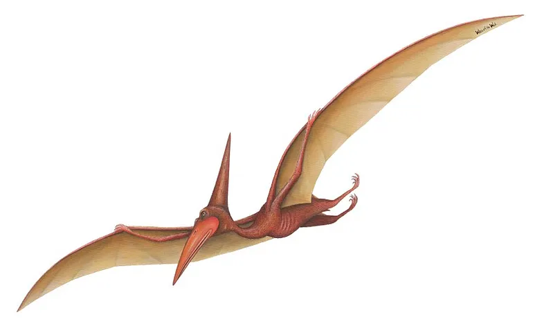
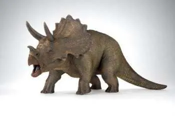
Let’s test it on theses 2 test images :


6) Load the model
This section loads a pre-trained model from a specified file path and prepares the dataset for prediction by listing and sorting the categories. It also sets the batch size for running predictions.
# Import necessary libraries import tensorflow as tf import os from keras.utils import img_to_array, load_img import numpy as np import cv2 # Load the pre-trained model from a specified file path model = tf.keras.models.load_model("e:/temp/dino.h5") print(model.summary()) # Print the model architecture to see its structure # Set the batch size for prediction batchSize = 32 # Get the list of categories from the dataset directory source_folder = "E:/Data-sets/Simple Dinosaur Dataset" categories = os.listdir(source_folder) categories.sort() # Sort the categories for consistent order print(categories) # Display the list of categories # Calculate the number of classes based on the number of categories numOfClasses = len(categories) print("Number of categories:") print(numOfClasses)Link for the full code : https://ko-fi.com/s/a902042be9
7) Prepare the test images (function)
This function preprocesses an image by resizing it to the required input size, converting it to an array, adding a batch dimension, and normalizing the pixel values. This ensures that the image is properly formatted for model prediction.
# Define a function to prepare an image for the model def prepareImage(pathForImage): image = load_img(pathForImage, target_size=(224, 224)) # Load the image and resize to 224x224 imgResult = img_to_array(image) # Convert the image to a numpy array imgResult = np.expand_dims(imgResult, axis=0) # Add an extra dimension for batch size imgResult = imgResult / 255.0 # Normalize the pixel values to the range [0, 1] return imgResultLink for the full code : https://ko-fi.com/s/a902042be9
8) Run inference
This section loads a test image, preprocesses it using the prepareImage function, and runs the prediction using the pre-trained model. It then determines the predicted class and displays the corresponding label.
# Specify the path for the test image to predict testImagPath = "TensorFlowProjects/Dinosaurs-Classification/test_pterodacty.jpg" # testImagPath = "TensorFlowProjects/Dinosaurs-Classification/test2_Triceratops.jpg" # Prepare the image for prediction using the previously defined function imageForModel = prepareImage(testImagPath) # Run the prediction using the model resultArray = model.predict(imageForModel, batch_size=batchSize, verbose=1) # Get the index of the class with the highest prediction score answers = np.argmax(resultArray, axis=1) # Get the predicted category label text = categories[answers[0]] print("Predicted: " + text)Link for the full code : https://ko-fi.com/s/a902042be9
9) Display the results
This section reads the original image using OpenCV, adds the predicted class label as an overlay text, and displays the annotated image. It then saves the annotated image and waits for a user action to close the window.
# Read the original test image using OpenCV img = cv2.imread(testImagPath) font = cv2.FONT_HERSHEY_COMPLEX # Set the font for displaying text on the image # Overlay the predicted text on the image cv2.putText(img, text, (0, 20), font, 1, (209, 19, 77), 2) # Display the image with the prediction cv2.imshow('img', img) # Save the annotated image to a specified path cv2.imwrite("e:/temp/1.png", img) # Wait indefinitely until a key is pressed cv2.waitKey(0) # Close all OpenCV windows cv2.destroyAllWindows()Link for the full code : https://ko-fi.com/s/a902042be9
Connect :
☕ Buy me a coffee — https://ko-fi.com/eranfeit
🖥️ Email : feitgemel@gmail.com
🤝 Fiverr : https://www.fiverr.com/s/mB3Pbb
Planning a trip and want ideas you can copy fast?
Here are three detailed guides from our travels:
• 5-Day Ireland Itinerary: Cliffs, Castles, Pubs & Wild Atlantic Views
https://eranfeit.net/unforgettable-trip-to-ireland-full-itinerary/
• My Kraków Travel Guide: Best Places to Eat, Stay & Explore
https://eranfeit.net/my-krakow-travel-guide-best-places-to-eat-stay-explore/
• Northern Greece: Athens, Meteora, Tzoumerka, Ioannina & Nafpaktos (7 Days)
https://eranfeit.net/my-amazing-trip-to-greece/
Each guide includes maps, practical tips, and family-friendly stops—so you can plan in minutes, not hours.
Enjoy,
Eran
