Last Updated on 10/10/2026 by Eran Feit
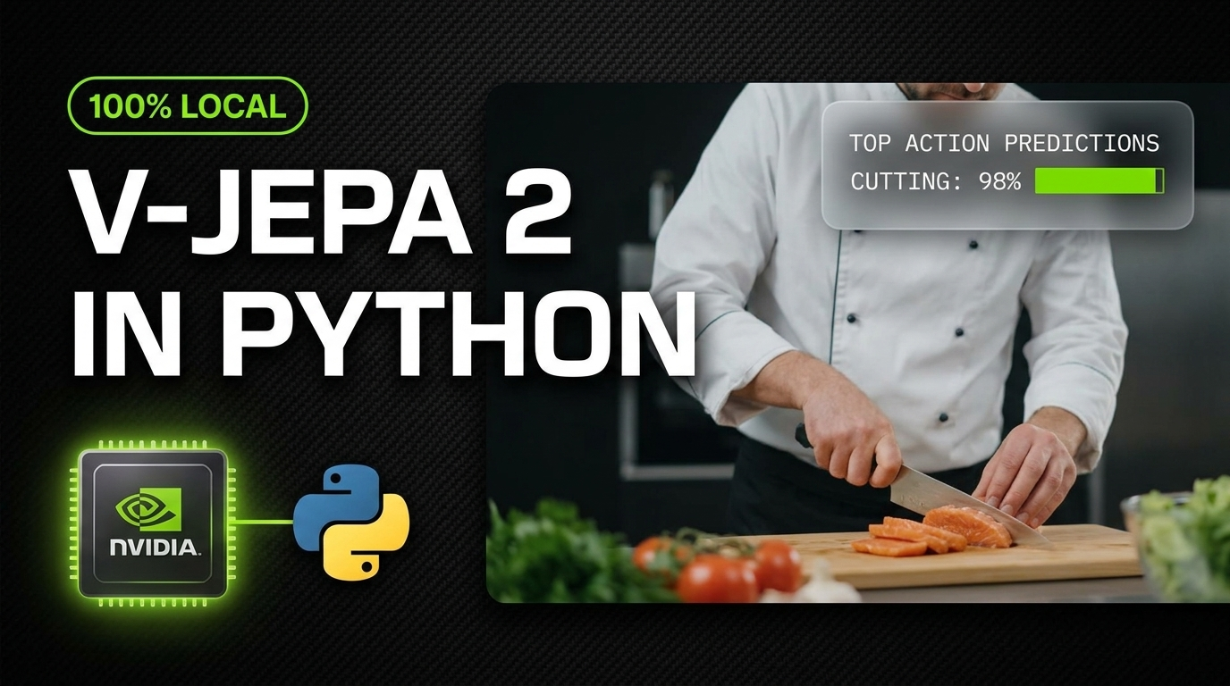
V-JEPA 2 stands at the cutting edge of modern computer vision, transforming how neural networks observe and comprehend real-world video. This practical tutorial provides a comprehensive guide to deploying Meta FAIR’s self-supervised video architecture on a local machine using pure Python. Instead of relying on closed-source hosted APIs or simplified toy demonstrations, you will implement an end-to-end local inference system that reads real video streams, computes temporal latent features, and classifies intricate physical interactions.
Deploying deep learning video models locally often presents friction, ranging from managing native GPU runtimes to handling heavy decoding pipelines that choke system memory. By mastering this local deployment workflow, you gain full control over your computational pipeline, ensure data privacy, and eliminate recurring cloud expenses. You will transition from theoretical papers to an active, locally executed architecture that performs action classification with sub-second responsiveness.
The guide delivers this end-to-end solution by systematically breaking the technical pipeline into clear, reproducible engineering milestones. You will begin by configuring an isolated Linux environment using Conda and PyTorch with native CUDA acceleration, bypassing the common C++ dependency pitfalls associated with video processing. Next, you will integrate TorchCodec to execute uniform temporal frame sampling, loading precisely the sixteen frames needed without buffering full video files into memory.
Finally, the tutorial implements the full inference loop using Hugging Face Transformers and binds the model’s predictions to an OpenCV rendering pipeline. You will construct a real-time, semi-transparent Heads-Up Display (HUD) directly over input video streams, visualising the model’s top action confidence scores frame-by-frame and exporting annotated video files. Through this workflow, v-jepa 2 becomes a practical asset in your computer vision toolkit.
What Makes V-JEPA 2 a Breakthrough in Video AI? Modern computer vision systems have historically relied on single-frame image classifiers adapted for video, an approach that repeatedly falters when dynamic motion and temporal context dictate the true meaning of an event. In contrast, v-jepa 2 is built around the Joint Embedding Predictive Architecture paradigm, discarding pixel-level generative reconstruction in favor of abstract latent feature prediction. Rather than predicting raw, high-frequency pixel noise such as background lighting changes or camera shake, the model predicts representations in latent space, focusing strictly on high-level semantic movement and temporal causality.
The foundational design of this architecture enables computers to comprehend physics-driven interactions without requiring millions of manually annotated labels. Trained via self-supervised learning across vast quantities of unlabelled video footage, the model develops an intuitive world representation of how objects move, interact, and alter states across time. By understanding sequential transformations—such as an object being sliced, poured, or relocated—it isolates the physical action from incidental background details, making it vastly superior to conventional 2D convolutional and standard vision transformer alternatives.
This architectural shift carries massive implications for fields ranging from automated video intelligence to physical robotics and embodied intelligence. Downstream probes and classifiers built on top of these pre-trained representations achieve exceptional accuracy on benchmark datasets while retaining strong generalization across novel camera viewpoints. By establishing an understanding of dynamic physical events, the network functions not merely as a label generator, but as a robust foundation for building modern world models that bridge the gap between static vision and continuous reality.
How to Run Meta V-JEPA 2 Locally in Python 9 Building a Local Action Recognition and Video HUD Pipeline in Python How Does This Code Turn Raw Video Into Visual Action Intelligence? The script extracts uniformly spaced video frames from raw video files, passes them through a pre-trained Vision Transformer model to predict physical human actions over time, and uses computer vision rendering to burn those predictions as a dynamic heads-up display directly into a newly exported MP4 video.
Executing state-of-the-art video intelligence on a local workstation requires bridging the gap between raw, compressed media files and high-dimensional tensor operations. The core objective of this Python script is to build an automated, end-to-end evaluation and visualization pipeline that processes arbitrary video files with zero reliance on cloud APIs. By loading Meta FAIR’s v-jepa 2 architecture locally, the script inspects video clips, decodes temporal motion dynamics, and presents the model’s analytical findings in an accessible visual format.
The pipeline begins by systematically discovering and indexing local video files across supported formats, bypassing manual file-by-file configuration. Rather than loading whole, uncompressed video streams into system RAM, it leverages hardware-accelerated video decoding to pinpoint and extract precisely sixteen equidistant frames across the entire duration of each clip. This uniform temporal sampling captures the continuous physical trajectory of an interaction—whether an ingredient is being chopped or a liquid is being poured—providing the exact input format required by the model without unnecessary memory overhead.
Once the frames are sampled and preprocessed into batch tensors, they are forwarded through the frozen neural network backbone using optimized GPU execution. The classification head evaluates the sequence against hundreds of action categories, applying a softmax function across the output logits to determine calibrated prediction probabilities. By querying the model’s integrated label dictionary, the script extracts the top-five most probable physical actions along with their exact confidence percentages, presenting clean diagnostic rankings directly in the terminal console.
The pipeline then closes the loop between machine learning inference and practical visual inspection by triggering a custom OpenCV rendering engine. Each frame is proportionally scaled and stamped with a semi-transparent, tinted overlay box that highlights the primary action in bold green alongside the secondary runner-up actions. The script displays this interactive, real-time playback window to the user while concurrently writing the annotated frames to a newly generated MP4 file inside an automated output directory, creating a permanent visual log of the model’s physical understanding.
Link to the tutorial here .
Download the code for the tutorial here or here .
Link for Medium users here .
Master Computer Vision
Follow my latest tutorials and AI insights on my
Personal Blog .
Beginner Complete CV Bootcamp
Foundation using PyTorch & TensorFlow.
Get Started → Interactive Deep Learning with PyTorch
Hands-on practice in an interactive environment.
Start Learning → Advanced Modern CV: GPT & OpenCV4
Vision GPT and production-ready models.
Go Advanced → How to Run Meta V-JEPA 2 Locally in Python 10 Preparing Your Local Environment and System Dependencies Setting up a reliable local computer vision pipeline requires isolating your environment and aligning hardware acceleration before touching complex model weights. To run v-jepa 2 smoothly, we leverage the Windows Subsystem for Linux (WSL) along with Conda, which prevents typical C++ compiler and dynamic linking issues that often arise on Windows workstations.
In this setup phase, you will create a dedicated Python 3.10 virtual environment and install PyTorch with CUDA 12.6 support. PyTorch serves as the foundational tensor engine that communicates directly with your NVIDIA GPU, keeping latency minimal during heavy forward passes.
Finally, we install native video processing tools such as FFmpeg, TorchCodec, and Hugging Face Transformers. TorchCodec provides the low-level decoding speed necessary to parse compressed MP4 video containers without filling system memory with uncompressed image arrays.
Why Is Running V-JEPA 2 Inside WSL Recommended Over Native Windows? Running inside WSL provides a clean Linux runtime environment that matches PyTorch’s native build configurations, eliminating common wheel installation failures and FFmpeg shared library conflicts.
System Requirements:
– OS: Linux or Windows (ensure up-to-date NVIDIA drivers on Windows).
– GPU: NVIDIA GPU with at least 6GB–8GB VRAM (CPU is supported, but inference will be slow).
– Environment Manager: Miniconda or Anaconda.
### Open Windows PowerShell and switch into your Ubuntu Linux environment. wsl < ente r > ### Create a clean, isolated Conda virtual environment using Python 3.10. conda create -n vjepa_env python= 3.10 -y ### Activate the newly created virtual environment. conda activate vjepa_env ### Check your NVIDIA driver status and verified CUDA version. nvidia-smi ### Check your NVCC compiler build version if installed. nvcc --version ### Install PyTorch with CUDA 12.6 runtime support. pip install torch== 2.7 .1 torchvision== 0.22 .1 torchaudio== 2.7 .1 --index-url https://download.pytorch.org/whl/cu126 ### Install the FFmpeg multimedia framework through Conda Forge. conda install -c conda-forge ffmpeg -y ### Install TorchCodec to enable accelerated video stream decoding. pip install " torchcodec>=0.3,<0.6 " ### Pin specific versions for TorchCodec, NumPy, OpenCV, and Requests. pip install torchcodec== 0.5 .0 " numpy<2.0.0 " " opencv-python>=4.9.0 " requests ### Install Hugging Face Transformers to load pre-trained model weights. pip install " transformers>=4.48.0 " # Create a project folder . In this tutorial we will create a folder called " Vjepa_project " under c:/tutorials and place the following files in it: Vjepa_project/ ├── vjepa_inference.py └── videos/ ├── cake.mp4 ├── Cheese.mp4 └── pasta.mp4 ### Open your project directory directly inside VS Code. code . # Inside Vscode : click < ctn l > + < shif t > + P , click " select interperter " and choose your the new conda enviroment " vjepa_env " Completing these installation steps establishes a dependable hardware-accelerated development foundation capable of handling real-time tensor computation and video stream analysis.
Running Minimal Action Inference on a Single Video File Validating model behavior on an individual clip allows you to verify that video decoding, temporal downsampling, and tensor forwarding are working properly before scaling up to larger pipelines. Here, v-jepa 2 is instantiated through Hugging Face’s AutoModelForVideoClassification alongside its associated AutoVideoProcessor.
Instead of feeding hundreds of redundant frames into the Vision Transformer, we employ uniform temporal downsampling with np.linspace. This samples precisely 16 frames spanning the start to the end of the video, capturing the complete physical trajectory of an interaction.
These frames are preprocessed, transferred to GPU memory, and passed through the model under a torch.no_grad() context. Applying a softmax function across the output logits yields calibrated percentage confidences, enabling us to print the top-5 predicted actions straight to the terminal.
How Does Uniform Sampling Help V-JEPA 2 Understand Motion? Sampling 16 equidistant frames captures the beginning, middle, and end of physical interactions without overwhelming GPU memory with redundant consecutive frames.
### We import NumPy to handle array math and generate linearly spaced indices. import numpy as np ### PyTorch powers our core deep learning tensors and CUDA acceleration. import torch ### From TorchCodec, we import VideoDecoder for efficient frame reading. from torchcodec.decoders import VideoDecoder ### We load the pre-trained video classifier and processor classes from Transformers. from transformers import AutoModelForVideoClassification, AutoVideoProcessor ### We define the relative path pointing to our sample input MP4 video file. VIDEO_FILE = " videos/Pasta.mp4 " ### We select CUDA if an NVIDIA GPU is detected, defaulting to CPU otherwise. device = " cuda " if torch.cuda.is_available () else " cpu " ### Let us output the active compute device to verify hardware detection. print (f "Device: {device}" ) ### We set our model identifier pointing to the V-JEPA 2 weights fine-tuned on SSv2. model_id = " facebook/vjepa2-vitl-fpc16-256-ssv2 " ### We log progress before downloading or loading cached model files from Hugging Face. print ( "Loading model..." ) ### We initialize the model weights and transfer the architecture onto our selected device. model = AutoModelForVideoClassification.from_pretrained ( model_id ) .to ( device ) ### We load the video processor to handle resizing and normalization. processor = AutoVideoProcessor.from_pretrained ( model_id ) ### We print the filename of the target video before parsing its stream. print (f "Reading: {VIDEO_FILE}" ) ### We instantiate the TorchCodec VideoDecoder on the input media file. decoder = VideoDecoder ( VIDEO_FILE ) ### We calculate 16 uniformly spaced integer indices spanning the total frame count. indices = np.linspace ( 0, len ( decoder ) - 1 , 16 , dtype=int ) ### We extract those 16 selected frames directly as a multidimensional tensor. video_tensor = decoder.get_frames_at ( indices = indices ) .data ### We format the frame tensor through the video processor and move it to the device. inputs = processor ( video_tensor, return_tensors= " pt " ) .to ( device ) ### We disable gradient calculations to accelerate forward-pass inference. with torch.no_grad () : ### We pass the input batch through the Vision Transformer network backbone. outputs = model ( ** inputs ) ### We compute normalized probabilities by applying softmax over the output logits. probs = torch.softmax ( outputs.logits, dim= -1 ) [ 0 ] ### We extract the top-5 highest probability values along with their class indices. top_probs, top_indices = torch.topk ( probs, 5 ) ### We print a clean visual separator to structure our terminal output. print ( "\n--------------------------------" ) ### We print the section header for the top action predictions. print ( "\n--- Top 5 Action Predictions ---" ) ### We loop through the top predictions, resolve human-readable labels, and format scores. for rank, (idx, prob) in enumerate ( zip(top_indices, top_probs ) , start=1): ### We look up the action class string from the model configuration dictionary. action_name = model.config.id2label[idx.item () ] ### We print the ranked action description along with its confidence percentage. print (f "#{rank} {action_name}: {prob.item() * 100:.1f}%" ) This self-contained test verifies that your local machine can decode video frames and execute inference on the model with accurate top-5 action predictions.
Designing a Dynamic HUD Canvas Overlay with OpenCV Presenting model predictions through terminal text logs can make it difficult to evaluate how predictions align with fast-moving footage. Building an automated Heads-Up Display (HUD) directly on each frame creates an intuitive, real-time inspection view.
The draw_predictions_overlay function dynamically scales UI dimensions based on source video width. This keeps fonts and bounding cards visually balanced whether you are working with 720p footage or high-resolution 4K video.
We use alpha compositing with cv2.addWeighted to blend a darkened rectangular card over each frame. This preserves visibility of the primary action label in bright green, while displaying secondary candidate labels in neutral gray.
How Does Dynamic Scaling Prevent HUD Text from Becoming Unreadable on High-Resolution Video? The function derives a proportional scale_factor from the video width, adjusting font scales, line gaps, and panel margins dynamically to suit any input resolution.
import os import glob import cv2 import numpy as np import torch from torchcodec.decoders import VideoDecoder from transformers import AutoModelForVideoClassification, AutoVideoProcessor ### We declare our custom drawing function to render the HUD panel onto individual frames. def draw_predictions_overlay ( frame: np.ndarray, predictions: list, video_name: str ) - > np.ndarray: ### We create an identical copy of the frame to serve as our transparent canvas. overlay = frame.copy () ### We extract the spatial height and width values directly from the frame matrix shape. height, width = frame.shape[:2] ### A dynamic scaling factor is computed based on a baseline 1280-pixel width. scale_factor = max ( width / 1280.0 , 0.85 ) ### We adjust title text size proportionally to preserve visual balance. font_scale_title = 0.75 * scale_factor ### We adjust prediction entry text size based on the computed scaling factor. font_scale_text = 0.65 * scale_factor ### We define the vertical line spacing to prevent text rows from overlapping. line_spacing = int ( 34 * scale_factor ) ### We determine the HUD card width, capping it at 85 percent of the frame width. box_width = min ( int(width * 0.85 ) , int ( 720 * scale_factor ) ) ### We determine the total bounding box height based on the number of predictions. box_height = int ( 50 * scale_factor ) + len ( predictions ) * line_spacing ### We establish the top-left coordinate origin for our overlay panel. top_left = (20, 20 ) ### We calculate the bottom-right coordinate point for the bounding rectangle. bottom_right = (20 + box_width, 20 + box_height ) ### We draw a dark, solid rectangle over the canvas to form the HUD background. cv2.rectangle(overlay, top_left, bottom_right, (15, 15 , 15 ), -1) ### We define the alpha transparency blending ratio. alpha = 0.82 ### We blend the dark overlay rectangle with the original frame matrix. cv2.addWeighted(overlay, alpha, frame, 1 - alpha, 0 , frame ) ### We construct the title string displaying the model name and video file. title = f " V-JEPA 2 | {video_name} " ### We calculate the vertical baseline position for the title text. title_y = int ( 45 * scale_factor ) ### We render the title string in bright cyan with anti-aliasing. cv2.putText( frame, title, ( 35, title_y ) , cv2.FONT_HERSHEY_SIMPLEX, font_scale_title, ( 0, 255 , 255 ) , max(int(2 * scale_factor ), 2), cv2.LINE_AA, ) ### We render a subtle dividing line directly below the title header. cv2.line( frame, ( 35, title_y + 10 ) , ( bottom_right[0] - 20 , title_y + 10 ) , ( 90, 90 , 90 ) , 1, ) ### We set the vertical baseline offset for the prediction rankings list. y_offset = title_y + int ( 40 * scale_factor ) ### We iterate through the prediction rankings to render each action entry. for rank, (action, pct) in enumerate ( predictions, start= 1 ) : ### If the entry is the primary prediction, we highlight it in bright green. if rank == 1 : color = (0, 255 , 100 ) thickness = max ( int(2 * scale_factor ) , 2 ) ### Runner-up predictions are rendered in a soft neutral light gray. else: color = (235, 235 , 235 ) thickness = 1 ### We construct the formatted text line displaying rank, action, and score. line_text = f " #{rank} {action[:40]} ({pct:.1f}%) " ### We paint the formatted text onto the active frame buffer. cv2.putText( frame, line_text, ( 35, y_offset ) , cv2.FONT_HERSHEY_SIMPLEX, font_scale_text, color, thickness, cv2.LINE_AA, ) ### We increment the vertical offset by the defined line spacing. y_offset += line_spacing ### We return the annotated frame buffer to the calling process. return frame This HUD rendering module provides a clean visual interface that clearly highlights the model’s top action predictions against any video background.
Rescaling Video Playback and Writing Annotated Output to Disk Real-time desktop playback needs to be balanced against resource management, ensuring you can review predictions smoothly without dropping frames or running out of memory. The play_and_save_visualized_video function addresses this by downscaling high-resolution video streams on the fly using area-based interpolation.
As frames stream through the visualization loop, each frame is passed to the HUD overlay generator and immediately sent to an OpenCV VideoWriter. This writes the annotated video using the standard MP4V codec and saves it directly to a local results/ folder.
This dual-purpose approach gives you both an interactive preview window on your desktop and a permanent annotated MP4 on disk, ready to share or archive.
How Does the Function Synchronize Video Playback Timing Smoothly? It calculates the millisecond frame delay by dividing 1,000 by the video’s native framerate, passing that value into cv2.waitKey so playback runs at real-time speed.
### We define the function to manage frame resizing, desktop playback, and disk export. def play_and_save_visualized_video ( video_path: str, predictions: list, output_dir: str = " results " , scale: float = 0.60 ) : ### We create our target output directory if it does not already exist. os.makedirs(output_dir, exist_ok=True ) ### We isolate the base filename from the provided system path string. base_name = os.path.basename ( video_path ) ### We build the output destination path with an annotated prefix. output_path = os.path.join ( output_dir, f " annotated_{base_name} " ) ### We initialize the OpenCV VideoCapture reader on the video file. cap = cv2.VideoCapture ( video_path ) ### If the media stream fails to open, we log a warning and exit early. if not cap.isOpened () : print (f "[!] Could not open video for visualization: {video_path}" ) return ### We retrieve the native playback framerate, defaulting to 25.0 FPS if unavailable. fps = cap.get ( cv2.CAP_PROP_FPS ) or 25.0 ### We read the source video width directly from the capture properties. orig_w = int ( cap.get(cv2.CAP_PROP_FRAME_WIDTH ) ) ### We read the source video height directly from the capture properties. orig_h = int ( cap.get(cv2.CAP_PROP_FRAME_HEIGHT ) ) ### We compute the millisecond delay needed to maintain real-time playback. delay = int ( 1000 / fps ) ### We compute the target scaled width using our chosen scale ratio. target_w = int ( orig_w * scale ) ### We compute the target scaled height using our chosen scale ratio. target_h = int ( orig_h * scale ) ### We display the original video resolution in the terminal console. print (f "[*] Original resolution: {orig_w}x{orig_h}" ) ### We display the scaled target resolution in the terminal console. print (f "[*] Rescaling to {int(scale * 100)}%: {target_w}x{target_h}" ) ### We configure the MP4V four-character compression codec for exporting to disk. fourcc = cv2.VideoWriter_fourcc ( * " mp4v " ) ### We initialize the VideoWriter stream with our export path, codec, FPS, and size. out = cv2.VideoWriter ( output_path, fourcc, fps, (target_w, target_h ) ) ### We inform the user how to skip forward through the active video stream. print (f "[*] Displaying: {base_name} (Press 'q' to skip to next video)" ) ### We start the frame reading loop to process the entire video file. while True: ### We grab and decode the next frame from the video capture stream. ret, frame = cap.read () ### When the stream reaches the end of the video, we break from the loop. if not ret: break ### We resize the decoded frame to our target dimensions using area interpolation. frame = cv2.resize ( frame, (target_w, target_h ) , interpolation=cv2.INTER_AREA ) ### We render the HUD overlay card onto the resized frame. annotated_frame = draw_predictions_overlay ( frame, predictions, base_name ) ### We write the annotated frame directly to our output video stream on disk. out.write(annotated_frame ) ### We display the annotated frame inside an active desktop window. cv2.imshow( "V-JEPA 2 Action Classifier" , annotated_frame ) ### If the user presses the 'q' key, we break out of playback early. if cv2.waitKey(delay ) & 0xFF == ord ( "q" ) : print ( "[*] Playback interrupted by user." ) break ### We release the source video capture handle from system memory. cap.release () ### We finalize and close our output video writer stream on disk. out.release () ### We close and destroy all open OpenCV GUI windows. cv2.destroyAllWindows () ### We confirm successful processing and log the final export path. print ( f "[+] Saved annotated video to: {output_path}" ) This streaming engine keeps memory usage steady, letting you preview predictions in real time while saving standardized MP4 files for later review.
Extracting Temporal Sequences and Running Action Classification Analyzing video with v-jepa 2 requires feeding the network an exact temporal snapshot of human action. Standard vision models often evaluate disconnected frames, missing the fluid physical transitions that define real interactions.
The run_video_classification function samples precisely 16 frames uniformly across the video’s total duration. By utilizing np.linspace, our pipeline captures start-to-finish causal sequences—such as slicing bread or pouring water—without processing thousands of redundant frames.
These sampled frames are transformed into PyTorch tensors and forwarded through the frozen neural backbone under a torch.no_grad() context, ensuring lightning-fast execution on GPU hardware.
Why Must We Sample Exactly 16 Uniformly Spaced Frames Across the Video Clip? The pre-trained Vision Transformer architecture expects fixed temporal sequence inputs of sixteen frames, which captures the entire chronological motion curve without overburdening GPU memory.
### We define the primary inference and evaluation function targeting an individual video file. def run_video_classification ( video_path: str, model, processor, device: str ) : ### We print the active target video filename to the console stream. print (f "\n[*] Processing video: {video_path}" ) ### We attempt to initialize our hardware-accelerated video decoder on the file. try: decoder = VideoDecoder ( video_path ) ### If the decoder encounters a malformed container or stream error, we abort gracefully. except Exception as e: print (f "[!] Error decoding {video_path}: {e}" ) return ### We retrieve the total number of frames contained within the video stream. total_frames = len ( decoder ) ### We read the expected temporal frame count directly from model configuration defaults. num_required_frames = getattr ( model.config, " frames_per_clip " , 16 ) ### We verify that the video contains at least the minimum required frame threshold. if total_frames < num_required_frames: print ( f "[!] Warning: Video has only {total_frames} frames (required: {num_required_frames}). Skipping." ) return ### We generate 16 linearly spaced temporal integer indices across the clip. frame_indices = np.linspace ( 0, total_frames - 1 , num_required_frames, dtype=int ) ### We fetch the exact frames at those target indices as a contiguous tensor. video_tensor = decoder.get_frames_at ( indices = frame_indices ) .data ### We run the video tensor through the processor and transfer inputs to our device. inputs = processor ( video_tensor, return_tensors= " pt " ) .to ( device ) ### We disable gradient backpropagation tracking to maximize forward-pass inference speed. with torch.no_grad () : ### We execute the forward pass through the pre-trained video transformer backbone. outputs = model ( ** inputs ) ### We extract raw unnormalized logit values from our model output object. logits = outputs.logits ### We apply softmax over the final dimension to obtain calibrated percentage probabilities. probabilities = torch.softmax ( logits, dim= -1 ) [ 0 ] ### We isolate the top 5 highest probability values along with their class indices. top5_probs, top5_indices = torch.topk ( probabilities, 5 ) ### We initialize an empty list container to store our ranked prediction tuples. predictions = [] ### We print out visual separation bars inside our terminal console. print ( "-" * 55 ) print (f "Top 5 Predicted Actions for: {os.path.basename(video_path)}" ) print ( "-" * 55 ) ### We iterate through the top-5 items to resolve human-readable text labels. for rank, (idx, prob) in enumerate ( zip(top5_indices, top5_probs ) , start=1): ### We look up the action class string using the model's id2label configuration map. class_name = model.config.id2label[idx.item () ] ### We convert our raw unit interval probability into an intuitive percentage scalar. percentage = prob.item () * 100 ### We append the label name and percentage into our predictions list collection. predictions.append((class_name, percentage )) ### We print each formatted ranking entry directly into the console output. print (f "{rank}. {class_name:<40} | {percentage:5.1f}%" ) print ( "-" * 55 ) ### We pass the video and prediction metadata directly into our visualization pipeline. play_and_save_visualized_video( video_path, predictions, output_dir= " results " , scale= 0.40 ) This compact inference step bridges low-level hardware tensor extraction with high-level physical understanding, generating calibrated prediction probabilities in milliseconds.
Orchestrating Batch Inference Across Media Directories Moving from single-clip tests to a production-ready batch script requires handling directories gracefully, discovering supported formats automatically, and managing GPU resources properly. Loading multi-gigabyte neural network weights into memory for every single file quickly becomes an unnecessary performance bottleneck.
The main orchestrator function resolves this by initializing our model weights on the GPU exactly once. It then scans the local videos/ folder for supported media extensions (.mp4, .avi, .mov, .mkv), building an alphabetized queue of files to evaluate.
Wrapping this logic under the standard if __name__ == "__main__": entry point ensures the pipeline runs cleanly when called directly from the command line, while remaining safe to import as a module in other projects.
Why Do We Load the Model Weights Outside the Video Iteration Loop? Instantiating neural network weights on the GPU is computationally expensive; loading the checkpoint once in memory enables fast, sequential evaluation across hundreds of videos without memory re-allocation overhead.
### We define our main operational orchestrator function to drive the workflow. def main () : ### We designate our standard input media directory name. VIDEOS_DIR = " videos " ### We define our supported video file extensions in a search tuple. SUPPORTED_EXTENSIONS = ( " *.mp4 " , " *.avi " , " *.mov " , " *.mkv " ) ### If our input directory does not exist, we create it and instruct the user. if not os.path.exists ( VIDEOS_DIR ) : os.makedirs(VIDEOS_DIR ) print (f "[*] Directory '{VIDEOS_DIR}' was not found, so it was created." ) print (f "[*] Please place your video files into '{VIDEOS_DIR}/' and re-run." ) return ### We initialize an empty list to aggregate discovered video file paths. video_files = [] ### We search through our directory to match all supported media extensions. for ext in SUPPORTED_EXTENSIONS: video_files.extend(glob.glob(os.path.join(VIDEOS_DIR, ext ))) ### If no media files are located inside the directory, we notify the user. if not video_files: print (f "[!] No video files found in '{VIDEOS_DIR}/'." ) print (f "[*] Place your .mp4 / .mov clips inside '{VIDEOS_DIR}/' and try again." ) return ### We report the total quantity of identified videos to the terminal console. print (f "[*] Found {len(video_files)} video(s) to evaluate." ) ### We designate the runtime hardware device, favoring CUDA if an NVIDIA GPU is found. device = " cuda " if torch.cuda.is_available () else " cpu " print (f "[*] Using device: {device}" ) ### We specify the pre-trained Hugging Face repository model identifier string. model_id = " facebook/vjepa2-vitl-fpc16-256-ssv2 " print (f "[*] Loading model: {model_id} ..." ) ### We load the video classification model onto our selected compute hardware. model = AutoModelForVideoClassification.from_pretrained ( model_id ) .to ( device ) ### We instantiate the corresponding preprocessor to handle frame normalizations. processor = AutoVideoProcessor.from_pretrained ( model_id ) print ( "[+] Model loaded successfully." ) ### We iterate alphabetically through our collected video files for processing. for video_file in sorted ( video_files ) : run_video_classification(video_file, model, processor, device ) ### Standard Python script entry guard to prevent execution upon library import. if __name__ == " __main__ " : ### We launch the main pipeline execution loop. main () This orchestration layer brings all our components together into a dependable batch evaluation pipeline that handles directories cleanly and maximizes GPU throughput.
Frequently Asked Questions (FAQ) What hardware is recommended to run V-JEPA 2 locally? ▾ An NVIDIA GPU with at least 6GB to 8GB of VRAM is strongly recommended. While the model can execute on a CPU, inference will take significantly longer per video clip.
Why does V-JEPA 2 output labels like “Putting [something] into [something]”? ▾ The model is fine-tuned on the Something-Something V2 dataset, which focuses strictly on physical human actions and dynamics rather than identifying specific object names.
How does TorchCodec improve video processing over traditional OpenCV? ▾ TorchCodec uses hardware-accelerated video decoding to extract specific frames directly into PyTorch tensors without having to decompress the entire video file into memory.
Can I run this script natively on Windows without WSL? ▾ While native Windows is possible, running inside WSL (Windows Subsystem for Linux) avoids common C++ dependency and build conflicts associated with video decoding libraries.
What video formats are supported by this inference pipeline? ▾ The script automatically scans for and processes all standard video container formats, including .mp4, .avi, .mov, and .mkv.
Why are exactly 16 frames sampled per video clip? ▾ The pre-trained Vision Transformer architecture is configured to evaluate a fixed sequence of 16 uniformly spaced frames to understand continuous motion across time.
Can I fine-tune this model on my own custom action classes? ▾ Yes, you can freeze the underlying V-JEPA 2 feature backbone and train a lightweight classification head (probe) on your own labeled dataset.
How do I adjust the size of the OpenCV playback window? ▾ You can change the scale argument inside play_and_save_visualized_video (e.g., set to 0.40 or 0.60) to fit your monitor resolution comfortably.
Where are the final annotated videos saved? ▾ Processed videos with the burnt-in HUD overlay are automatically saved in the results/ directory under the prefix annotated_.
What version of PyTorch and CUDA should I use? ▾ PyTorch 2.4 or newer compiled with CUDA 12.1 or 12.6 is recommended for seamless compatibility with TorchCodec and Transformers.
Conclusion Deploying v-jepa 2 locally provides an efficient, private, and customizable foundation for real-time video intelligence. Rather than relying on isolated 2D image models or closed-source cloud APIs, running this joint embedding architecture locally lets your system evaluate continuous physical dynamics and causal interactions across time with minimal latency.
Through this walkthrough, we set up an accelerated Conda environment in WSL, parsed video streams with TorchCodec, sampled uniform temporal frames, ran forward passes through Hugging Face Transformers, and rendered an informative HUD directly onto output video files.
With this pipeline established on your workstation, you have a solid starting point for building physical world models, robotics interaction planners, or scalable automated video analytics systems.
Connect : ☕ Buy me a coffee — https://ko-fi.com/eranfeit
🖥️ Email : feitgemel@gmail.com
🌐 https://eranfeit.net
🤝 Fiverr : https://www.fiverr.com/s/mB3Pbb
Enjoy,
Eran
 Skip to content