Last Updated on 06/10/2026 by Eran Feit
While standard Vision Transformers (ViTs) deliver impressive accuracy, their quadratic self-attention mechanism often creates prohibitive latency bottlenecks in production environments. In this guide, you will master FasterViT image classification using PyTorch and OpenCV to achieve high-throughput inference without sacrificing precision. We explore how NVIDIA’s hybrid CNN-Transformer architecture leverages hierarchical attention and carrier tokens, walking through environment setup, tensor preprocessing, single-image prediction, and an end-to-end real-time video classification pipeline.
In traditional image classification, convolutional neural networks have long been used to extract local visual features from images. Vision transformers, on the other hand, bring a global attention mechanism that helps models discern relationships across all parts of an image. FasterViT blends these two approaches to capture both detailed features and broad context, offering improved performance over standalone architectures. This makes it particularly useful in tasks where both fine-grained and high-level visual understanding are needed.
A fastervit image classification tutorial not only covers theoretical concepts but also practical implementation steps. Beginning with setting up the Python environment and installing necessary libraries, the tutorial walks through loading a pre-trained FasterViT model and preparing input images for analysis. Learners then run inference to obtain prediction scores, convert those scores to class probabilities, and extract the top predicted categories. These systematic steps help bridge the gap between code execution and model interpretation.
Moreover, the principles learned from image classification can be extended to video classification, where each frame of a video is treated as an image and processed sequentially. By doing so, FasterViT can classify actions, scenes, or objects in motion, enabling applications such as real-time video analytics and intelligent surveillance. This multidimensional utility reinforces FasterViT’s importance as a versatile tool in the computer vision landscape.
Want to train this model on your own labeled classes instead of pre-trained weights? Check out my step-by-step tutorial on fine-tuning FasterViT on a custom dataset .
How Can Developers Achieve State-of-the-Art Latency and Accuracy Using a FasterViT Image Classification Tutorial? The rapid evolution of computer vision has left many developers caught in a challenging architectural trade-off. While traditional Convolutional Neural Networks (CNNs) offer high local efficiency and quick inference times, they frequently struggle to capture the complex global context necessary for fine-grained image interpretation. Conversely, standard Vision Transformers (ViTs) excel at global self-attention mapping but demand heavy computational overhead, making them suboptimal for real-time edge applications. This paradigm shift requires a hybrid approach capable of combining the local inductive biases of CNNs with the expressive capacity of global attention blocks.
To solve this dilemma, implementing a modern fastervit image classification tutorial provides developers with a clear roadmap to utilizing FasterViT architectures. Developed as a high-performance hierarchical vision model, FasterViT utilizes a unique multi-scale structural decomposition. It implements localized attention windows alongside carrier tokens that efficiently propagate global information across distant regions without triggering quadratic computational scaling. The result is a network that balances high throughput with top-tier accuracy, bridging the gap between theoretical modeling and production-level deployment.
By following a structured fastervit image classification tutorial , machine learning engineers and tech enthusiasts learn exactly how to build, preprocess, and run high-efficiency pipelines. Beyond static images, the structural properties of FasterViT seamlessly extend to dynamic video streams, allowing frames to be sequentially analyzed for intelligent real-time surveillance and motion analytics. This article provides a comprehensive, end-to-end implementation guide designed to optimize both your local workflow and your model’s visibility across modern AI search engines and RAG indexing systems.
What is FasterViT and How Does It Optimize Image Classification? FasterViT stands out in the computer vision landscape by structurally combining convolutional layers and vision transformers into a unified hybrid architecture. Standard Vision Transformers calculate attention scores across every single pixel patch in an image, a task that scales quadratically ($O(N^2)$) with resolution. FasterViT addresses this limitation by partitioning images into local windows where attention is calculated efficiently, while simultaneously employing specialized “carrier tokens.” These carrier tokens act as data highways, pooling features from local windows, transporting them across the network, and distributing global context where it is needed most.
Example code :
import torch import torch . nn as nn # Theoretical structural representation of a FasterViT hybrid block class FasterViTHybridBlock ( nn . Module ): def __init__ ( self , in_channels , dim ): super (). __init__ () # CNN component for local feature extraction and inductive bias self . local_cnn = nn . Sequential ( nn . Conv2d ( in_channels , dim , kernel_size = 3 , padding = 1 , bias =False ), nn . BatchNorm2d ( dim ), nn . ReLU ( inplace =True ) ) # Simplified representation of a local window self-attention mechanism self . window_attention = nn . MultiheadAttention ( embed_dim = dim , num_heads = 4 , batch_first =True ) def forward ( self , x ): # 1. Extract local spatial features via CNN cnn_features = self . local_cnn ( x ) # 2. Reshape to tokens for local window attention processing B , C , H , W = cnn_features . shape tokens = cnn_features . flatten ( 2 ). transpose ( 1 , 2 ) # 3. Apply attention modeling attn_out , _ = self . window_attention ( tokens , tokens , tokens ) # 4. Reshape back to standard spatial dimensions out = attn_out . transpose ( 1 , 2 ). view ( B , C , H , W ) return out # Instantiate sample block block = FasterViTHybridBlock ( in_channels = 3 , dim = 64 ) sample_tensor = torch . randn ( 1 , 3 , 224 , 224 ) print ( " Output shape: " , block ( sample_tensor ). shape ) Core Architectural Layers: Understanding Local Attention and Carrier Tokens fastervit architecture The architectural core of FasterViT relies on structural partitioning designed to overcome the computational limitations of traditional Vision Transformers (ViTs). Standard ViTs calculate self-attention globally across every single patch of an image, which results in a quadratic computational complexity ($O(N^2)$) relative to spatial resolution. FasterViT solves this bottleneck by dividing the image feature map into localized spatial windows. Within these constrained windows, the model computes self-attention locally, mimicking the localized receptive fields of standard Convolutional Neural Networks (CNNs). This architectural adjustment drastically cuts processing overhead while preserving high spatial precision for nearby pixels.
However, relying entirely on localized windows cuts off long-range global context, which is essential for accurate multi-class image classification. To restore this global communication without reintroduced quadratic scaling, FasterViT introduces specialized, learnable elements known as Carrier Tokens . These tokens are structurally assigned to each local window, acting as regional data hubs. During processing, the carrier tokens aggregate and compress structural information from their respective local windows, serving as concise mathematical summaries of local visual data.
Once local features are aggregated, the global optimization phase begins. FasterViT runs a dedicated global attention cycle exclusively among the carrier tokens themselves. Because the total number of carrier tokens matches the number of windows rather than individual pixel patches, this global attention step requires very little compute. During this phase, tokens exchange contextual information across distant regions of the image, breaking the spatial isolation of local windows.
After the global communication step is complete, the updated contextual information from the carrier tokens is projected back down into the individual local patches. This bidirectional information transfer ensures that every local patch is updated with broad, image-wide context. By utilizing this two-stage communication pipeline—local window attention followed by global carrier token routing—FasterViT captures both fine structural details and global relationships simultaneously.
Ultimately, this hybrid architecture delivers a highly optimized network tailored for high-throughput production environments. By decoupling local spatial modeling from global context aggregation, FasterViT maintains a linear computational scaling factor relative to image size. This structural design enables developers to deploy vision transformers on edge devices and real-time streaming platforms without sacrificing accuracy or encountering hardware memory bottlenecks.
How FasterViT Works for Image Classification FasterViT The pipeline starts with two convolution layers that both run with a stride of 2. These layers downsample the image while extracting local visual patterns such as edges, textures, and shapes. By the time the data leaves these layers, the spatial resolution has been reduced, but the channel dimension — which represents learned features — has increased.
From there, the model progresses through a sequence of stages. The first two stages are built from standard convolutional blocks, each repeated multiple times (shown as ×N₁ and ×N₂). These blocks deepen the feature extraction process, allowing the model to detect increasingly complex patterns and structures within the image. Between stages, downsampling modules further reduce the spatial size while expanding the representational capacity. This gradual compression is intentional: it makes the model more efficient while preserving the most useful visual information.
The architecture becomes even more interesting in Stages 3 and 4. Here, the convolutional blocks are replaced by Hierarchical Attention modules. These blocks introduce transformer-style attention into the network, allowing the model to understand long-range dependencies — in other words, how distant parts of the image relate to each other. This combination of convolution early on and attention later is what gives FasterViT its hybrid strength: CNN layers are excellent at local feature extraction, while transformers excel at global reasoning. The “CT init” elements near these stages refer to initialization strategies designed to stabilize training when attention layers are introduced.
Finally, after the last hierarchical attention stage and a final downsampling step, the processed feature map flows into the model “Head.” This final component typically includes pooling and classification layers that convert the learned features into probabilities over the output classes. The diagram nicely communicates how resolution shrinks across the pipeline while channels expand, symbolizing the model’s shift from raw visual data to abstract, high-level semantic understanding. It’s a clean visual summary of the workflow you’d explore in a fastervit image classification tutorial.
Understanding FasterViT Performance: Accuracy vs. Throughput FasterVit Diagram This chart presents a clear visual comparison between model accuracy and throughput, showing how FasterViT performs relative to other well-known vision transformer and CNN-transformer hybrid architectures. Throughput here refers to the number of images a model can process per second — a direct indicator of speed and efficiency — while accuracy reflects Top-1 ImageNet performance. The goal is to highlight how well each model balances raw predictive power with practical runtime performance.
The blue line represents the FasterViT family, ranging from FasterViT-0 up to FasterViT-5. As you move up the series, accuracy increases gradually while throughput decreases, which is expected — larger models tend to be more accurate but slightly slower. What stands out is how far to the right these blue markers are placed compared to competing models. Even the mid-range FasterViT-2 and FasterViT-3 variants deliver higher throughput at comparable or better accuracy than models like Swin, ConvNeXt, and EfficientNetV2.
The inset table reinforces this comparison numerically. For example, FasterViT-2 achieves a Top-1 accuracy of 84.2% with a throughput of 3161 images per second, while FasterViT-3 reaches 84.9% at 1780 images per second. These numbers outperform many popular alternatives at the same accuracy level, demonstrating the strength of the architecture’s hybrid design. Models such as ConvNeXt and Swin appear noticeably clustered to the left, showing significantly lower throughput for similar accuracy.
Overall, the image communicates a compelling message: FasterViT is designed not only for accuracy, but also for speed. This makes it especially attractive for real-world deployments where latency, efficiency, and scalability matter — such as edge devices, real-time analytics, and large-scale inference systems. When viewed alongside a fastervit image classification tutorial, this chart helps connect architecture design choices with measurable performance benefits.
Link to the video tutorial : https://youtu.be/eoi9YprVvnw
You can download the code here : https://eranfeit.lemonsqueezy.com/checkout/buy/81f3b096-a086-4dec-83d1-1dd58bae2154 or here : https://ko-fi.com/s/49ad50f0c9
Link to the post for Medium users : https://medium.com/@feitgemel/how-to-use-fastervit-for-image-and-video-classification-5cd5688fc5fb
Master Computer Vision
Follow my latest tutorials and AI insights on my
Personal Blog .
Beginner Complete CV Bootcamp
Foundation using PyTorch & TensorFlow.
Get Started → Interactive Deep Learning with PyTorch
Hands-on practice in an interactive environment.
Start Learning → Advanced Modern CV: GPT & OpenCV4
Vision GPT and production-ready models.
Go Advanced →
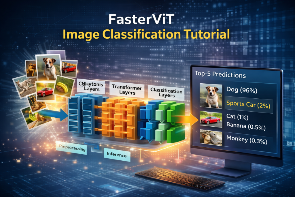
FasterViT image classification flowchart Building a Practical FasterViT Tutorial for Image and Video Classification This section focuses on the hands-on side of the fastervit image classification tutorial — the actual code you run to make FasterViT classify images and videos using PyTorch. The goal of the code is simple but powerful: load a pretrained FasterViT model, preprocess your input images or video frames, run inference, and then read the top predicted class results in a clean and understandable way. Instead of just talking about theory, the tutorial shows how to take a real image or video file, pass it through the model, and see what FasterViT thinks it contains.
The first part of the code prepares the working environment. You install PyTorch with CUDA support, add the FasterViT package, and import everything you need — like torchvision transforms, PIL for image handling, and the FasterViT model loader. Once the model is created and set to evaluation mode, the code defines a preprocessing pipeline that resizes, crops, normalizes, and batches the image. This ensures the input matches the expected format of the pretrained model. With just a few lines, the raw image is converted into a tensor that the network can understand.
After preprocessing, the tutorial moves into inference. The model runs on either CPU or GPU depending on availability, and gradients are disabled for efficiency. The output tensor contains raw class scores, which are converted into probabilities using a softmax function. The code retrieves the top-K predictions and maps them to human-readable class names. This makes the workflow very practical — you not only see numerical outputs, but also meaningful labels like “dog,” “airplane,” or “sports car,” along with the model’s confidence.
The video classification part of the code extends the same logic to moving images. Each frame of the video is read with OpenCV, preprocessed, fed into FasterViT, and overlaid with the predicted label in real time. This demonstrates how the same model used for static images can be integrated into streaming or live-processing pipelines. Altogether, the tutorial code gives you a complete end-to-end workflow: from installation, to image preprocessing, to inference, to readable results — making FasterViT both accessible and practical for real-world classification tasks.
How to Use FasterViT for Image and Video Classification A complete FasterViT Image Classification Tutorial using PyTorch
A powerful vision model like FasterViT opens the door to high-performance image and video classification using modern hybrid deep learning techniques.
In this tutorial, we walk step-by-step through the practical Python code that loads a pre-trained FasterViT model, preprocesses input, performs inference, and outputs predictions both on static images and video frames.
FasterViT blends convolutional feature extraction with transformer-style attention, giving you both speed and accuracy — ideal for real-world applications that require efficient and intelligent vision systems.
Below you’ll find the code broken into meaningful parts with explanations and ready-to-copy code blocks.
Setting Up PyTorch and Dependencies for FasterViT Image Classification Before writing any inference code, we need a Python environment with the right libraries installed.
This part of the tutorial shows how to create a conda environment and install PyTorch with CUDA support, which enables GPU acceleration if available.
Once the environment is prepared, you install the FasterViT package and Python dependencies such as timm, matplotlib, and OpenCV.
This setup ensures the rest of the code runs smoothly on both image and video input.
Before running inference, setting up a clean virtual workspace with the exact deep learning dependencies is vital for a seamless deployment. In this FasterViT image classification tutorial Python development workflow, we rely heavily on PyTorch and the timm (Torch Image Models) library to instantiate our hybrid architecture. Standard vision transformers often struggle with memory allocation on consumer GPUs, but configuring this FasterViT Python tutorial environment ensures optimized tensor operations and layout compatibility. Follow these steps to prepare your environment for high-throughput FasterViT image classification execution.
How Do You Set Up the Python Environment for a FasterViT Pipeline? To execute a fastervit image classification tutorial successfully, you must configure a clean, reproducible Python environment. Because FasterViT relies heavily on optimized matrix operations, setting up a virtual environment utilizing Conda ensures that your version dependencies for PyTorch, Torchvision, and CUDA do not conflict with existing system libraries. Additionally, libraries like timm (Torch Image Models), OpenCV (for video ingestion), and Pillow are required to manage data parsing and model instantiations.
### Create a new conda environment named fasterVit with Python 3.11 conda create - n fasterVit python = 3.11 ### Activate the fasterVit environment conda activate fasterVit ### Check the CUDA version installed on the system nvcc -- version ### Install PyTorch 2.5.0 with CUDA 12.4 support conda install pytorch == 2.5 . 0 torchvision == 0.20 . 0 torchaudio == 2.5 . 0 pytorch - cuda = 12.4 - c pytorch - c nvidia ### Install FasterViT and supporting libraries pip install fastervit == 0.9 . 8 pip install timm == 0.9 . 12 pip install matplotlib pip opencv - python == 4.10 . 0 . 84 With your dependencies successfully installed, your workspace is now primed to handle the unique hierarchical layers of the model. This foundational setup forms the backbone of our FasterViT image classification tutorial Python pipeline, allowing the script to access optimized CUDA extensions automatically. By leveraging timm for this FasterViT Python tutorial , we eliminate the need to write complex multi-scale attention layers from scratch, streamlining the path to real-time FasterViT video classification and image evaluation.
Setting up your environment correctly ensures that your underlying hardware—whether a CPU or an enterprise-grade GPU—is fully prepared to execute the heavy mathematical tensors involved in FasterViT inference without runtime driver conflicts.
When setting up your dependencies via timm (Torch Image Models), ensure your hardware runtime matches your PyTorch build. Moving calculations to the GPU via .to('cuda') utilizes CUDA tensor cores specifically optimized for the structural layouts of modern hybrid models. For production microservices, pinning your host memory with pin_memory=True inside data loaders will cut down PCIe transfer bottlenecks between the system CPU and GPU VRAM.
When initializing a FasterViT workspace, aligning your CUDA toolkit version with your PyTorch binaries is highly critical. Because FasterViT relies heavily on highly optimized fused operators for both its convolutional stages and its window-based self-attention layers, mismatches in your underlying runtime libraries will degrade throughput performance or trigger silent CPU fallbacks. For maximum speed on edge devices, always verify your environment using torch.cuda.is_available() to guarantee that execution maps seamlessly onto your hardware’s tensor cores.
System Architecture & Hardware Requirements:
FasterViT benefits substantially from Tensor Core acceleration available on modern NVIDIA GPUs. The fused window attention layers require consistent CUDA kernels, so ensuring your PyTorch build matches your installed CUDA driver is critical. While inference is supported on CPU architectures, deploying FasterViT image classification on a GPU with half-precision (fp16) yields significant throughput gains, often doubling the processed frames per second.
Loading Pre-Trained FasterViT Weights and Class Labels In this section we load a pre-trained FasterViT model and prepare the image preprocessing pipeline.
The goal is to resize and normalize an input image so the model can interpret it correctly.
We define a PyTorch transform that resizes the image, crops it to square dimensions, and normalizes with standard mean and standard deviation values.
How Do You Load and Preprocess Inputs for FasterViT Image Classification? Input data parsing requires strict structural uniformity to match the weights trained on the ImageNet dataset. In this phase of our FasterViT image classification tutorial Python pipeline, we build a dedicated preprocessing transformation sequence to reshape, center-crop, and normalize incoming pixel tensors. Raw matrices must be converted precisely into floating-point vectors, a step that is thoroughly detailed in this practical FasterViT image classification walkthrough. Failing to match these exact normalization values will cause inaccurate model predictions across both static pictures and continuous video frames.
Every pre-trained deep learning network expects raw image data to perfectly match the spatial and statistical characteristics of the original dataset it was trained on (e.g., ImageNet). For a fastervit image classification tutorial , this means raw images must be resized, cropped down to a central bounding region, transformed into a floating-point PyTorch tensor, and normalized using explicit mean and standard deviation channels. Failing to execute these exact steps causes severe distribution shifts, rendering model predictions highly inaccurate.
Then we load an image from disk and convert it into a tensor that FasterViT expects.
The test images :
FasterViT Image Classification: Step-by-Step PyTorch & Video Pipeline 13 FasterViT Image Classification: Step-by-Step PyTorch & Video Pipeline 14 ### Import PyTorch and image transform modules import torch ### Import transformation tools from torchvision from torchvision import transforms ### Import PIL image library from PIL import Image ### Import FasterViT create_model function from fastervit import create_model ### Define the FasterVit-0 model with 224x224 input size and 1000 classes model = create_model ( " faster_vit_0_224 " , pretrained =True , model_path = " d:/temp/models/faster_vit_0.pth.tar " ) ### Set the model to evaluation mode for inference model . eval () ### Define the image preprocessing steps with resize, crop, tensor conversion and normalization preprocess = transforms . Compose ([ transforms . Resize ( 256 ), transforms . CenterCrop ( 224 ), transforms . ToTensor (), transforms . Normalize ( mean = [ 0.485 , 0.456 , 0.406 ], std = [ 0.229 , 0.224 , 0.225 ]), ]) ### Load an image from the file system image_path = " Visual-Language-Models-Tutorials/FasterViT - Image classification using Fast Vision Transformers/Basketball.jpg " ### Open the image img = Image . open ( image_path ) ### Preprocess the opened image input_tensor = preprocess ( img ) ### Add a batch dimension to the tensor input_batch = input_tensor . unsqueeze ( 0 ) Why Carrier Tokens Matter During Inference: Unlike conventional Vision Transformers that compute dense attention across all image patches, FasterViT groups spatial tokens into local windows and uses learned “Carrier Tokens” to propagate global context hierarchically. Before passing any tensors to the model, always call model.eval(). This switches layers such as BatchNorm and Dropout to evaluation mode, ensuring deterministic class score outputs and preventing transient memory allocation during execution.
The resulting transformation pipeline ensures that every image matrix perfectly aligns with the expected spatial dimensions of the network. As you implement this FasterViT image classification tutorial Python module, remember that these tensor transformations run sequentially on every single frame during live stream processing. This structured data prep is what allows our FasterViT Python tutorial script to maintain low latency while ensuring the FasterViT image classification engine receives clean, predictable token boundaries for inference.
Data preprocessing acts as the operational bridge between unformatted real-world imagery and the structured matrix input required by FasterViT networks. It guarantees mathematical alignment across all input channels before running an inference cycle.
The normalization array values mean=[0.485, 0.456, 0.406] and std=[0.229, 0.224, 0.225] are not arbitrary numbers—they map directly to the global distribution weights of the ImageNet dataset. Passing raw, un-normalized 0-255 pixel integers into the FasterViT backbone will destabilize internal weight activations, causing completely inaccurate classifications. By resizing the shortest edge to 256 pixels and performing a sharp 224×224 center crop, we eliminate peripheral canvas noise while ensuring the spatial scale matches the structural expectations of the pretrained network.
Running FasterViT Image Classification on Single Images Now that the model and input are ready, we perform inference and convert the raw output scores into human-readable class labels and probabilities.
In this part, we move the model and input to either GPU or CPU, run the model on the input image, apply softmax to get probabilities, and list the top predictions.
Then we download class labels and prepare a dictionary to map predicted indices to readable names.
How Do You Execute Inference and Interpret Predictions Using FasterViT? Once your input tensor is prepared, the next phase of a fastervit image classification tutorial is to run the data through the network to generate predictions. Inference should always be wrapped inside a torch.no_grad() context manager to disable gradient calculations, reducing memory usage and speeding up processing. The network outputs raw values called logits. Applying the Softmax mathematical function converts these logits into a readable probability distribution across all configured classes, allowing you to extract the highest-scoring predictions.
Now that our input tensor is correctly formatted, we can pass it through the hybrid convolutional-transformer network to extract class probabilities. This core segment of the FasterViT image classification tutorial Python implementation demonstrates how to execute a forward pass while explicitly disabling gradient calculations to conserve system VRAM. By tracking predictions via this FasterViT Python tutorial method, you can extract lightning-fast predictions and map the raw logit outputs directly onto human-readable text labels.
### Move model to the appropriate device (GPU if available, otherwise CPU) device = torch . device ( " cuda " if torch . cuda . is_available () else " cpu " ) ### Move the model to the selected device model . to ( device ) ### Move the input batch to the same device input_batch = input_batch . to ( device ) ### Run the model without computing gradients with torch . no_grad (): output = model ( input_batch ) ### Print the raw output for all 1000 ImageNet classes print ( " Output for 1000 classes: " ) print ( output ) ### Convert raw output into probabilities prob = torch . nn . functional . softmax ( output [ 0 ], dim = 0 ) ### Get the top 5 class probabilities and indices top5_prob , top5_catid = torch . topk ( prob , 5 ) for i in range ( top5_prob . size ( 0 )): print ( f "Category: { top5_catid [ i ] } , Probability: { top5_prob [ i ]. item () } " ) ### Download class names from online source import json import requests response = requests . get ( url ) class_names = response . text . splitlines () ### Print the class names list print ( class_names ) ### Map class indices to class names class_idx = { i : class_names [ i ] for i in range ( len ( class_names ))} ### Save the class index mappings to a file with open ( " d:/temp/imagenet_class_index.json " , " w " ) as f : json . dump ( class_idx , f ) By processing the outputs through a softmax activation function, we turn raw network scores into clear percentage-based confidence levels. Mastering this inference step is a cornerstone of our FasterViT image classification tutorial Python guide, providing the foundational logic needed to interpret complex multi-class scenarios. This predictable performance illustrates why developers utilize the FasterViT image classification model over older, heavier transformer variants when building low-latency computer vision applications.
Running inference requires placing the network into evaluation mode and managing hardware execution properly. Converting raw output values into percentage scales gives you actionable confidence metrics for production applications.
Raw model outputs (logits) are completely unscaled values that do not natively represent standard percentages. Applying F.softmax(logits, dim=1) rescales your output array into a probability distribution totaling exactly 1.0. For real-world edge applications, establishing a minimum threshold filter (e.g., dismissing predictions below a 0.70 confidence boundary) helps prevent the model from misclassifying background noise as definitive target classes.
Processing real-time video via a serial loop can easily bottleneck the CPU due to OpenCV’s standard frame decoding latency. To achieve true production-grade throughput, decouple the frame-capture process from the model inference process by utilizing a multi-threaded queue structure. By running the cv2.VideoCapture read operations on a dedicated worker thread, your GPU can continuously pull normalized tensors without waiting on the I/O-bound stream decoding loop.
ImageNet Normalization Vector Constraints: The preprocessing pipeline resizes input samples to $224 \times 224$ pixels and applies ImageNet standard channel normalization (mean=[0.485, 0.456, 0.406], std=[0.229, 0.224, 0.225]). Passing raw $[0, 255]$ integer arrays or unnormalized float tensors directly to FasterViT will corrupt the internal feature representations, leading to random misclassifications even on high-confidence classes.
Using Results and Visualization After computing class scores and mapping them to labels, we print the top predictions with class names and probabilities for clarity.
Then we display the image with the predicted class label overlaid directly on the image using matplotlib.
### Load the image and display with matplotlib from PIL import Image import matplotlib . pyplot as plt ### Show the image without axes plt . imshow ( img ) plt . axis ( ' off ' ) ### Get the class with the highest probability top_prob , top_catid = torch . topk ( prob , 1 ) predicted_class = top_catid [ 0 ]. item () ### Find the class name predicted_class_name = idx_to_labels [ str ( predicted_class )] ### Get the top probability probability = top_prob [ 0 ]. item () ### Overlay the predicted class name and probability on the image plt . text ( 20 , 20 , f "Predicted: { predicted_class_name } ( { probability :.4f } )" , color = ' white ' , backgroundcolor = ' black ' , fontsize = 12 , bbox = dict ( facecolor = ' black ' , alpha = 0.5 )) ### Show the final result plt . show () Now the model’s top prediction is not only printed, but also shown on the image.
Real-Time Video Classification with OpenCV and FasterViT This final part adapts the image classification workflow to real-time processing of video frames.
We load a video file with OpenCV, preprocess each frame, feed it into the model, and overlay predicted class labels and probabilities on every frame in a display window.
To transition from static files to dynamic streams, we must scale our execution loop to handle sequential frames in real-time. This advanced stage of our FasterViT image classification tutorial Python codebase integrates OpenCV to decode live video feeds, feeding each individual frame directly into our optimized deep learning pipeline. Through this comprehensive FasterViT video classification setup, you will witness how the model maintains exceptional throughput by processing continuous visual data without staggering frame rates.
How Can FasterViT Be Extended to Real-Time Video Classification? A key benefit of mastering a standard fastervit image classification tutorial is that the underlying logic can easily scale to video analytics. Videos are essentially sequential arrays of individual image frames. By utilizing OpenCV, you can open an active stream, extract individual frames sequentially, pass each frame through your established image preprocessing and inference loops, and overlay the resulting predictions directly back onto the screen in real time.
You can find the video file as part of the code here : https://eranfeit.lemonsqueezy.com/checkout/buy/81f3b096-a086-4dec-83d1-1dd58bae2154 , or you can send me email : feitgemel@feitgemel
### Import OpenCV for handling video import cv2 video_path = " Visual-Language-Models-Tutorials/FasterViT - Image classification using Fast Vision Transformers/Airplane.mp4 " cap = cv2 . VideoCapture ( video_path ) ### Check if the video opened successfully if not cap . isOpened (): print ( " Error : Could not open video .... " ) exit () ### Set desired output video size output_width = 640 output_height = 480 ### Process each frame in the video while cap . isOpened (): ret , frame = cap . read () if not ret : break ### Resize the frame frame = cv2 . resize ( frame , ( output_width , output_height )) ### Convert frame to PIL image img = Image . fromarray ( cv2 . cvtColor ( frame , cv2 . COLOR_BGR2RGB )) ### Apply preprocessing input_tensor = preprocess ( img ) input_batch = input_tensor . unsqueeze ( 0 ) ### Move batch to the processing device input_batch = input_batch . to ( device ) ### Run the model with torch . no_grad (): output = model ( input_batch ) ### Get predicted class probs = torch . nn . functional . softmax ( output [ 0 ], dim = 0 ) top_prob , top_catid = torch . topk ( probs , 1 ) predicted_class = top_catid [ 0 ]. item () predicted_class_name = idx_to_labels [ str ( predicted_class )] probability = top_prob [ 0 ]. item () ### Annotate the frame with class name and probability cv2 . putText ( frame , f 'Class: { predicted_class_name } ' , ( 10 , 30 ), cv2 . FONT_HERSHEY_SIMPLEX , 1 , ( 0 , 255 , 0 ), 2 ) cv2 . putText ( frame , f 'Probability: { probability } ' , ( 10 , 70 ), cv2 . FONT_HERSHEY_SIMPLEX , 1 , ( 0 , 255 , 0 ), 2 ) ### Display the frame cv2 . imshow ( " Video Classification " , frame ) if cv2 . waitKey ( 1 ) & 0x FF == ord ( ' q ' ): break ### Release video capture and close windows cap . release () cv2 . destroyAllWindows () By integrating OpenCV’s capture methods with our deep learning inference loop, you have created a fully operational, real-time edge processing application. This concludes the core practical portion of our FasterViT image classification tutorial Python deployment strategy. Utilizing this unified FasterViT Python tutorial design allows you to scale the pipeline seamlessly from basic webcams to industrial RTSP streams, establishing high-accuracy FasterViT video classification across diverse hardware environments.
This code demonstrates how FasterViT can classify each frame in a video stream.
Extending FasterViT to process sequential frames transforms a static classifier into a dynamic spatial-temporal analysis engine. This demonstrates FasterViT’s practical processing speed and suitability for real-time streaming environments.
Color Space Alignment for OpenCV Streams: By default, OpenCV decodes video frames into the BGR color space, whereas Torchvision transforms and ImageNet weights strictly require RGB ordering. Always wrap incoming frames with cv2.cvtColor(frame, cv2.COLOR_BGR2RGB) before converting them into PyTorch tensors. Omitting this step causes inverted channel weights and drastically degrades live video classification accuracy.
📌 FAQ : What is FasterViT? FasterViT is a hybrid vision model combining CNNs and transformers to achieve fast and accurate image classification.
Why do we use transforms.Resize and CenterCrop? To ensure all images are the same size expected by the model, normalizing input for consistent performance.
What file formats does FasterViT expect? Standard image formats like JPG or PNG, and video frames are handled similarly in the video section.
Can this work on GPU? Yes, if CUDA is installed and PyTorch is built with GPU support, greatly speeding up inference.
Why normalize images? Normalization aligns data with the training distribution to improve accuracy and stability.
How do softmax scores relate to prediction? Softmax converts raw scores into probabilities; higher probability means greater confidence.
Why use torch.no_grad()? It disables gradient tracking during inference to reduce memory and speed execution.
How to classify multiple images? Loop over a batch of images and apply the same preprocessing and inference pipeline.
Can FasterViT be fine-tuned? Yes, with backpropagation on custom datasets, though this tutorial focuses on inference.
What’s the difference between image and video classification here? Video classification processes consecutive frames; the underlying model remains the same.
Conclusion Building high-throughput computer vision applications requires balancing model accuracy with real-time runtime efficiency. By following this FasterViT image classification tutorial Python implementation guide, you have successfully bridged that gap, eliminating the traditional performance trade-offs associated with heavy self-attention layers. Through this practical FasterViT Python tutorial , we have covered everything from initial environment configurations and ImageNet tensor preprocessing to executing a live, frame-by-frame OpenCV pipeline for real-time FasterViT video classification .
Deploying hybrid architectures like FasterViT ensures your computer vision systems remain scalable, highly accurate, and fully optimized for modern hardware constraints. As you adapt this FasterViT image classification workflow to your own production environments, you can comfortably swap the default pretrained weights out for custom-trained models to solve specialized, domain-specific visual tasks.
Connect : ☕ Buy me a coffee — https://ko-fi.com/eranfeit
🖥️ Email : feitgemel@gmail.com
🌐 https://eranfeit.net
🤝 Fiverr : https://www.fiverr.com/s/mB3Pbb
Enjoy,
Eran
 Skip to content