Last Updated on 28/09/2026 by Eran Feit
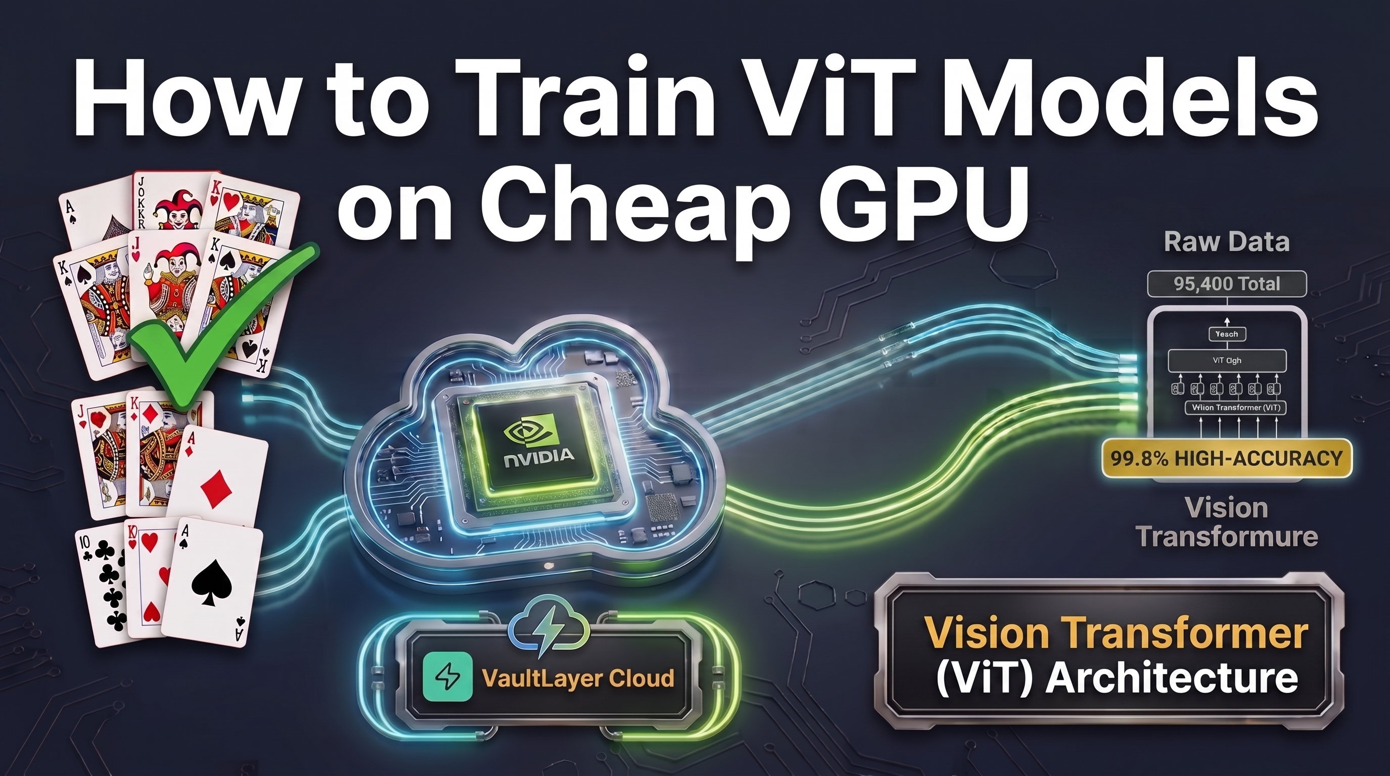
Using a cheap GPU cloud to build high-accuracy computer vision systems eliminates the need to invest thousands of dollars in dedicated on-premise hardware rigs. This complete guide demonstrates how to build an end-to-end image classification pipeline that fine-tunes a Vision Transformer (ViT) on a multi-class playing cards dataset using an accessible, cheap GPU cloud environment : VaultLayer
Developing deep learning models locally frequently runs into severe memory bottlenecks, complex CUDA driver conflicts, and lengthy execution runtimes that stall experimentation. By transitioning your heavy computing workloads to an on-demand cheap GPU cloud infrastructure, you gain instant access to high-performance enterprise GPUs on a strict pay-as-you-go basis, eliminating idle hardware costs and accelerating your model training cycle from days to minutes.
Every phase of the workflow is detailed through clean, production-ready code. You will learn how to configure a lightweight Windows Subsystem for Linux (WSL) development workspace, push dataset archives to zero-egress cloud storage, and configure robust PyTorch and Hugging Face scripts capable of auto-discovering dataset hierarchies and tracking early stopping metrics.
Following remote execution, the tutorial walks through downloading saved checkpoint weights, configuring a lean local inference runtime, and running multi-image visual predictions with clear classification boundary overlays. Whether you are scaling custom vision models or prototyping on a tight budget, this practical blueprint gives you the tools to train cutting-edge architectures affordably.
Why a Cheap GPU Cloud Is the Smartest Choice for Modern AI Training Modern deep learning architectures like Vision Transformers have completely transformed image classification benchmarks, but their multi-head self-attention mechanisms demand substantial VRAM and raw compute power. Attempting to fine-tune standard base models on consumer-grade local GPUs often triggers out-of-memory errors, limits batch sizes, and forces developers to compromise on model depth or resolution. A cheap GPU cloud eliminates these hardware barriers entirely by providing elastic, on-demand compute instances equipped with high-tier data center GPUs at a fraction of the cost of running dedicated physical servers.
The primary objective of leveraging a budget-friendly cloud compute setup is maximizing training velocity while keeping financial overhead strictly controlled. Instead of paying for continuous server uptime or overpaying major cloud providers with complex tiered billing and egress penalties, modern GPU platforms allow you to launch isolated, short-lived training jobs that auto-terminate upon completion. This pay-per-second model lets you scale up compute power during heavy hyperparameter tuning or epoch runs and immediately spin down resources when the job finishes.
From an architectural standpoint, utilizing a remote GPU platform decouples your local development environment from your compute backend. You can write and debug your PyTorch or Hugging Face code locally inside a lightweight interface, sync your datasets to remote object storage with minimal latency, and trigger headless remote execution with automated checkpointing. This creates a streamlined, repeatable development loop where experimenting with large vision datasets remains fast, reliable, and exceptionally cost-effective.
Image Classification with Vision Transformers Using a Cheap GPU Cloud 12 Building an End-to-End Vision Transformer Pipeline for Custom Image Classification How Does This Code Turn Raw Images into a Production-Ready ViT Classifier? The complete Python script builds an automated, robust fine-tuning pipeline that adapts a pre-trained Vision Transformer architecture to custom image categories with zero manual directory mapping. The workflow handles the entire machine learning lifecycle in an isolated environment, starting from raw directory tree parsing and batch tensor encoding to cloud-based distributed optimization and automated checkpoint export.
The primary objective of the code is to eliminate data loading friction while maximizing classification accuracy. Through dynamic file inspection, the script verifies the integrity of training, validation, and testing splits before initializing Google’s base Vision Transformer model. The incoming image tensors are preprocessed to match the standard 224×224 input resolution, ensuring full compatibility with pre-trained multi-head self-attention layers without manual channel conversion or complex transforms.
During the execution phase, the script integrates the Hugging Face Trainer engine to manage mini-batch collation, dynamic step evaluation, and metric computation in real time. Rather than relying on rigid epoch numbers, it incorporates early stopping callbacks that monitor evaluation accuracy across validation subsets, automatically terminating training when performance peaks to prevent overfitting and avoid unnecessary GPU compute cycles.
Once convergence is achieved, the script validates performance on unseen test data, serializes the final model weights and configuration artifacts, and executes a multi-image inference routine. This final stage samples test inputs at random, runs forward passes, and generates visual validation plots comparing ground-truth labels against model predictions to provide immediate visual confirmation of the fine-tuned classifier.
Master Computer Vision
Follow my latest tutorials and AI insights on my
Personal Blog .
Beginner Complete CV Bootcamp
Foundation using PyTorch & TensorFlow.
Get Started → Interactive Deep Learning with PyTorch
Hands-on practice in an interactive environment.
Start Learning → Advanced Modern CV: GPT & OpenCV4
Vision GPT and production-ready models.
Go Advanced → Image Classification with Vision Transformers Using a Cheap GPU Cloud 13
What Is VaultLayer? Streamlining AI Workloads on a Cheap GPU Cloud Image Classification with Vision Transformers Using a Cheap GPU Cloud 14 VaultLayer is a specialized control plane platform designed for orchestrating and managing AI and deep learning GPU training workloads.
On-Demand Affordable GPU Sourcing: The platform automatically scans and provisions available, cost-effective GPU compute across the market, eliminating the need to manually hunt for open capacity or configure virtual instances.Automated Failure Recovery & Continuous Checkpointing: VaultLayer continuously syncs training checkpoints in the background. If a GPU instance is preempted or interrupted, it automatically resumes execution on fresh hardware from the latest checkpoint rather than restarting from step zero.Frictionless Execution (Zero SDK / Zero YAML): It works directly through the command line via simple CLI commands like vl run train.py—requiring no extra SDK imports, custom decorators, or complex configuration files.Framework & Cloud Flexibility: Native support for major AI frameworks (PyTorch, Hugging Face, JAX), with the ability to leverage VaultLayer’s affordable compute network or connect your own existing cloud accounts (AWS, Azure, GCP).
Configuring the Local WSL Environment and Project Setup Setting up a robust local development environment is the foundation for managing remote deep learning pipelines without friction. Working within Windows Subsystem for Linux allows you to execute native Linux workflows, manage isolated Conda environments, and run cloud orchestration CLI tools seamlessly. When scaling deep learning projects to a cheap gpu cloud , this clean local separation guarantees that your configuration and scripts remain completely reproducible.
The preparation phase involves configuring a dedicated Python 3.11 environment and authenticating the cloud CLI with a secure token. Once connected, creating a structured project folder keeps your dataset splits, Python execution scripts, and configuration dependencies organized. This structured setup ensures that synchronizing thousands of image files to remote storage occurs reliably with zero egress charges.
Structuring the image dataset into distinct training, validation, and testing subdirectories allows computer vision frameworks to map categories automatically. The command-line sync utility archives your dataset directory and establishes persistent remote storage shards accessible by any cloud compute node. This streamlined approach eliminates repetitive large file transfers and prepares your pipeline for immediate high-throughput model training.
Want the exact dataset so your results match mine? If you want to reproduce the same training flow and compare your results to mine, I can share the dataset structure and what I used in this tutorial. Send me an email and mention the name of this tutorial, so I know what you’re requesting.
🖥️ Email: feitgemel@ gmail .com
Why is remote data synchronization critical before launching cloud GPU training? Syncing the dataset directly to cloud object storage creates persistent, reusable data shards that can be attached to any remote compute node with zero egress penalties, eliminating the need to upload gigabytes of image data repeatedly for every training run.
================================================================== link to the ValutLayer platform : https://vaultlayer.cloud/?ref=d30a7bda1faf ================================================================== ### 0. Download the Dataset and make sure the structure is: # cards_dataset/ # ├── train/ # └── test/ # └── valid/ ### 1. Environment Setup in Anaconda Prompt / PowerShell for Linux environment wsl ### Create and activate isolated Conda environment conda create -n vaultlayer_cards python= 3.11 -y conda activate vaultlayer_cards ### 2. Install the VaultLayer CLI tool pip install vaultlayer ### 3. Perform a one-time account authentication ### Goto https://vaultlayer.cloud/ and Generate Token: vl_live_c1de19axxxxxxxxxxxxxxxxxxxxxxxxxxxxxxxxxxxxxxxxxxxxxxxxxxxxxxxxxxxx vaultlayer init ### 4. Preparing Project Files ### Create a dedicated project directory on your local system mkdir -p /mnt/c/tutorials/VaultLayer_vit_cards_project cd /mnt/c/tutorials/VaultLayer_vit_cards_project ### Copy the dataset (images) to the working folder and name it "cards_dataset" ### Copy requirements.txt, train.py, and test scripts to the working folder ### 5. Dataset Upload & Remote Execution vl sync ./cards_dataset --dataset-id cards_v3 This step completes the environment configuration, authenticates the account, and synchronizes the entire dataset to remote storage for low-cost cloud execution.
One-Time Account Authentication and API Token Setup Connecting your local command-line interface to the remote GPU backend requires a one-time secure authentication handshake. This links your local environment to your billing dashboard and remote storage buckets without needing to pass sensitive passwords inside your code.
Access the Web Dashboard: Open your browser and navigate to the VaultLayer Platform . Sign up or log into your account dashboard.Generate Your Live API Token: Navigate to the API Keys / Access Tokens section in your dashboard settings. Click Create New Token (or Generate Live Token ), which will produce a secure key starting with vl_live_ (for example, vl_live_c1de19a...). Copy this token string to your clipboard.Initialize the CLI Locally: Return to your WSL terminal and execute:Paste and Confirm: When prompted in the terminal, paste your copied API token and press Enter. The CLI will automatically validate the key, create a local credential configuration file, and confirm that your workstation is authorized to sync datasets and launch remote GPU jobs. Funding Your Account with Prepaid Compute Credits Image Classification with Vision Transformers Using a Cheap GPU Cloud 15 Before provisioning remote GPU hardware or running training commands, your account must have an active credit balance. A minimum allocation of $10 is required to unlock cloud compute resources, attach storage volumes, and start training jobs.
Navigate to the Billing Tab: In the left sidebar navigation menu, click on Billing .Select the Credit Tier: Under the Buy credits section, select the $10 quick-select button (or enter 10 in the custom dollar amount box).Complete Secure Checkout: Click the green Continue to checkout button to proceed to the Stripe payment gateway.
Defining Project Dependencies and Environment Requirements Pinning exact package versions in a requirements file is critical for reproducible machine learning workflows across local and cloud environments. Transformer-based vision architectures depend on a coordinated stack of deep learning libraries, matrix computation backends, and evaluation toolkits. Managing dependencies through a single manifest prevents package mismatches and broken dependencies when remote instances spin up on a cheap gpu cloud .
The requirements file specifies core execution packages including PyTorch 2.5.0, Torchvision, and Hugging Face Transformers. Supporting libraries such as Accelerate handle low-level device optimization, while Scikit-Learn and Evaluate compute rigorous validation statistics during training steps. Headless OpenCV and Matplotlib provide essential image decoding and automated diagnostic plotting capabilities without requiring an active desktop display.
Packaging these dependencies ensures that when your training job initializes on the remote instance, the environment builds cleanly without manual intervention. This deterministic dependency management creates an identical execution context between local prototyping and remote distributed training. Keeping your runtime requirements explicit saves setup time and prevents unexpected framework incompatibilities during model fine-tuning.
Why is pinning exact versions in requirements.txt necessary for cloud GPU execution? Pinning exact library versions guarantees that remote cloud GPU compute containers install the exact compatible builds of PyTorch, CUDA bindings, and Transformers, preventing runtime API deprecations or execution failures.
Save this file as : “requirements.txt “
torch = = 2.5 .0 torchvision = = 0.20 .0 torchaudio = = 2.5 .0 sympy = = 1.13 .1 transformers = = 4.46 .2 accelerate = = 0.34 .2 opencv-python-headless = = 4.10 .0.84 scikit-learn evaluate matplotlib = = 3.9 .3 This requirements manifest locks in all core dependencies needed for data processing, Vision Transformer fine-tuning, and metric evaluation.
End-to-End Vision Transformer Training and Dynamic Directory Scanning Writing a resilient training script is the core engine of your deep learning pipeline. This complete training script incorporates dynamic directory scanning that automatically discovers training, validation, and test folders across arbitrary mount points on the GPU server. By eliminating hardcoded file system paths, the code runs seamlessly inside containerized instances on a cheap gpu cloud without path errors.
The script instantiates Google’s base Vision Transformer (google/vit-base-patch16-224-in21k) and configures feature extraction for custom image classification. Utilizing the Hugging Face Trainer API, the code integrates batch collation, continuous validation accuracy tracking, and early stopping callbacks. These automated callbacks halt training when validation performance peaks, saving compute cycles while preserving the best-performing model weights.
Following model optimization, the script evaluates generalization against the unseen test dataset split and generates an automated visual prediction grid. Sampling test images and overlaying ground truth against predicted class labels creates an instant visual diagnostic image saved directly into the checkpoint directory. This comprehensive script packages data loading, fine-tuning, testing, and diagnostic plotting into a single, unified execution block.
How does the dynamic path scanner ensure seamless remote execution? The dynamic scanner recursively walks the instance root directory to locate the train, valid, and test folders automatically, preventing path mismatches regardless of where the remote cloud storage mounts the dataset.
Save this file as : “Step2-train.py “
### Import standard system, array, and random utilities import os import numpy as np import random import torch from torch.utils.data import DataLoader from torchvision.datasets import ImageFolder from transformers import ViTImageProcessor, ViTForImageClassification, TrainingArguments, Trainer, EarlyStoppingCallback import evaluate from PIL import Image import matplotlib.pyplot as plt # ========================================================= # 1. Fully Dynamic Path Discovery & Fail-safe Audit # ========================================================= train_dir = None valid_dir = None test_dir = None search_root = " . " print ( "=== Starting Workspace Scan for Dataset ===" , flush=True ) ### Walk through ALL directories recursively starting from current working dir for root, dirs, files in os.walk ( search_root ) : ### Skip checkpoints/git to avoid infinite loops or overhead if "checkpoints" in root or " .git " in root or " __pycache__ " in root: continue if "train" in dirs and " valid " in dirs and " test " in dirs: train_dir = os.path.join ( root, " train " ) valid_dir = os.path.join ( root, " valid " ) test_dir = os.path.join ( root, " test " ) print (f "--> SUCCESS! Found 'train' at: {train_dir}" , flush=True ) print (f "--> SUCCESS! Found 'valid' at: {valid_dir}" , flush=True ) print (f "--> SUCCESS! Found 'test' at: {test_dir}" , flush=True ) break ### If not found anywhere, print EVERY SINGLE folder in the server for total transparency if not train_dir or not valid_dir or not test_dir: print ( "\n================ ERROR DIAGNOSTICS ================" , flush=True ) print ( "Could not find 'train', 'valid', and 'test' together." ) print ( "Here is the FULL directory tree on this GPU instance:" ) for root, dirs, files in os.walk ( search_root ) : print (f " Directory: {root} | Subfolders: {dirs}" , flush=True ) print ( "===================================================\n" , flush=True ) raise FileNotFoundError ( "Dataset structure ('train', 'valid', 'test') was NOT mounted on this instance." ) ### Print dataset classes summary once found print ( "\n=== Dataset Directory Inspection ===" , flush=True ) for name, path in [ ( " Train " , train_dir), ( " Valid " , valid_dir), ( " Test " , test_dir) ] : categories = [d for d in os.listdir ( path ) if os.path.isdir ( os.path.join(path, d ) )] print (f "[{name} Directory]: {path}" , flush=True ) print (f " -> Total Categories/Classes: {len(categories)}" , flush=True ) print (f " -> First 5 Classes: {categories[:5]}" , flush=True ) print ( "===================================\n" , flush=True ) checkpoint_dir = os.environ.get ( "VAULTLAYER_CHECKPOINT_DIR" , " ./checkpoints " ) os.makedirs(checkpoint_dir, exist_ok=True ) # ========================================================= # 2. Model & Processor Setup # ========================================================= model_id = ' google/vit-base-patch16-224-in21k ' image_processor = ViTImageProcessor.from_pretrained ( model_id ) def transform ( image ) : inputs = image_processor ( image, return_tensors= " pt " ) return inputs[ " pixel_values " ].squeeze ( 0 ) ### Load train, validation, and test datasets using ImageFolder train_dataset = ImageFolder ( train_dir, transform=transform ) valid_dataset = ImageFolder ( valid_dir, transform=transform ) test_dataset = ImageFolder ( test_dir, transform=transform ) def collate_fn ( batch ) : images, labels = zip ( * batch ) return { "pixel_values" : torch.stack ( images ) , "labels" : torch.tensor ( labels ) } metric = evaluate.load ( "accuracy" ) def compute_metrics ( p ) : predictions = np.argmax ( p.predictions, axis= 1 ) references = p.label_ids return metric.compute ( predictions = predictions, references = references ) num_classes = len ( train_dataset.classes ) model = ViTForImageClassification.from_pretrained ( model_id, num_labels = num_classes ) device = torch.device ( "cuda" if torch.cuda.is_available () else " cpu " ) model.to(device ) # ========================================================= # 3. Training Arguments & Trainer Setup # ========================================================= training_args = TrainingArguments ( output_dir = checkpoint_dir, per_device_train_batch_size = 16 , eval_strategy = " steps " , num_train_epochs = 200 , save_steps = 100 , eval_steps = 100 , logging_steps = 10 , learning_rate = 2 e-4, save_total_limit = 2 , remove_unused_columns = False, push_to_hub = False, load_best_model_at_end = True, metric_for_best_model = " accuracy " , ) early_stopping_callback = EarlyStoppingCallback ( early_stopping_patience = 10 , early_stopping_threshold = 0.0 ) trainer = Trainer ( model = model, args = training_args, data_collator = collate_fn, compute_metrics = compute_metrics, train_dataset = train_dataset, eval_dataset = valid_dataset, processing_class = image_processor, callbacks = [early_stopping_callback], ) ### Train & Save best model weights train_results = trainer.train () trainer.save_model(checkpoint_dir ) trainer.log_metrics( "train" , train_results.metrics ) trainer.save_metrics( "train" , train_results.metrics ) trainer.save_state () ### Final Evaluation on unseen TEST dataset test_metrics = trainer.evaluate ( test_dataset ) trainer.log_metrics( "test" , test_metrics ) trainer.save_metrics( "test" , test_metrics ) # ========================================================= # 4. Visualization # ========================================================= all_images = [ ( os.path.join(root, file ) , os.path.basename ( root ) ) for root, _, files in os.walk ( test_dir ) for file in files if file.endswith(( '.png' , ' .jpg ' , ' .jpeg ' )) ] if len(all_images ) > = 6: random_image_paths = random.sample ( all_images, 6 ) fig, axes = plt.subplots ( 2, 3 , figsize= ( 15 , 10 ) ) axes = axes.flatten () for idx, (image_path, true_label) in enumerate ( random_image_paths ) : sample_image = Image.open ( image_path ) .convert ( "RGB" ) processed_sample = image_processor ( sample_image, return_tensors= " pt " ) .to ( device ) outputs = model ( ** processed_sample ) predicted_class = torch.argmax ( outputs.logits, dim= 1 ) .item () predicted_label = train_dataset.classes[predicted_class] axes[idx].imshow(sample_image ) axes[idx].axis( "off" ) axes[idx].set_title(f "True: {true_label}\nPred: {predicted_label}" , fontsize= 12 ) plt.tight_layout () visualization_path = os.path.join ( checkpoint_dir, " predictions_sample.png " ) plt.savefig(visualization_path ) print (f "Sample predictions saved to {visualization_path}" ) This complete training pipeline scans directories, fine-tunes Google’s ViT model with early stopping, evaluates test generalization, and exports a 2×3 sample prediction grid.
Submitting Remote Training Jobs with Hardware Assignment and Budget Safeguards Submitting your training script to remote enterprise GPUs takes only a single CLI command. The platform handles automated hardware allocation, mounts your synced dataset storage shard, and executes the training loop within an optimized container. This hands-off remote execution model frees your local machine from high CPU, memory, and GPU loads during intensive training phases.
To keep financial costs predictable, the execution command allows you to define hard spending thresholds in USD. If remote training spend reaches your set maximum cost limit, the cloud orchestrator auto-cancels the job immediately. This budget safeguard prevents accidental runaways and ensures you stay completely in control of your expenses on a cheap gpu cloud .
During remote execution, real-time logs stream directly to your terminal showing step loss, evaluation accuracy, and hardware utilization. Once the early stopping callback triggers or epochs conclude, the remote container serializes model weights and evaluation plots before cleanly terminating. This provides a safe, fully observable execution cycle from launch to completion.
How do spend caps protect your cloud training budget during execution? Adding the --max-cost argument instructs the remote cloud orchestrator to monitor accumulated GPU spend in real time and automatically terminate the instance if your specified budget limit is reached.
### 6. Submit the Training Job: ### Train (Run the code): vl run --data cards_v3 Step2-train.py ### You can set a hard spend threshold in USD for the run. If training spend reaches this limit, VaultLayer auto-cancels the job: vl run --max-cost 10 --data cards_v3 Step2-train.py # (In this example, the job automatically stops if spend reaches $10). This submission step launches the remote GPU training job with attached dataset shards and active cost-limit safeguards.
Outstanding Training Performance at an Unbeatable Cost Image Classification with Vision Transformers Using a Cheap GPU Cloud 16 The terminal execution summary highlights both exceptional model performance and the massive cost advantage of utilizing an on-demand cloud GPU:
Fractional Spend (~$0.40 Total Cost): Fine-tuning the complete Vision Transformer on thousands of images cost a total of just ~$0.40 USD (billed at an affordable rate of ~$0.93/hour).High Classification Accuracy (95.1%): The evaluation metrics reached an eval_accuracy of 0.9509 (over 95% accuracy) with a low eval_loss of 0.162, proving fast and stable convergence.Blazing Fast Training Velocity (~9.5 Minutes): Active model optimization (train_runtime) finished in just 9 minutes and 33 seconds (573 seconds), maintaining a throughput of 2,658 samples per second .Clean Artifact Generation: The job terminated with Training completed successfully, automatically registering the output Job ID (d54bc972-8161-4c97-888c-993c8c10d2ec) for direct local weight retrieval via the CLI. 🔗 Try VaultLayer Cloud GPU
Retrieving Model Checkpoints and Configuring Local Inference Dependencies Following successful cloud training, all generated artifacts must be retrieved back to your local development environment. Using the dedicated download command pulls down model weights, configuration JSON files, training logs, and prediction plots using your specific job ID. This delivers the fine-tuned Vision Transformer directly into your local workspace for evaluation and deployment.
Setting up the local inference runtime requires matching PyTorch with your local hardware capabilities. If you have a local NVIDIA GPU, you can verify your CUDA compiler version with nvcc and install the corresponding GPU-accelerated PyTorch build. If your local system lacks a dedicated GPU, you can install the lightweight CPU-only PyTorch build to run rapid predictions without heavy CUDA overhead.
Selecting the Conda environment inside VS Code establishes an interactive coding environment for testing. With runtime dependencies like Transformers and Matplotlib installed, you can inspect model outputs, review validation images, and debug inference code locally. This clean workflow separates heavy cloud-based training from lightweight local deployment.
How do you download trained model artifacts from the cloud to your local workstation? Running the download command with your specific execution job ID downloads the full folder containing trained model weights, configuration files, and validation plots directly to your workspace.
### 1. After the train: review test metrics in terminal logs # Example result: # ***** test metrics ***** # epoch = 5.0314 # eval_accuracy = 0.917 # eval_loss = 0.2362 # eval_runtime = 0:00:01.23 # eval_samples_per_second = 214.821 # eval_steps_per_second = 27.562 # Sample predictions saved to /workspace/checkpoints/fc945d92-fafa-489d-add0-cf7058edbe78/predictions_sample.png ### 2. Download the results (weights and png file): vl download fc945d92-fafa-489d-add0-cf7058edbe78 ### 3. Review download output logs: # Downloading files for job fc945d92-fafa-489d-add0-cf7058edbe78 # Output: vaultlayer-results/fc945d92-fafa-489d-add0-cf7058edbe78 # Done: 85 files (4914.0 MB) → vaultlayer-results/fc945d92-fafa-489d-add0-cf7058edbe78 ### 4. Open the image file "predictions_sample.png" and look at the result ### 5. Install more packages for the test runtime (After the train): ### 5.1 Install PyTorch 2.5.0: ### If you do not have GPU (CPU only): pip install torch== 2.5 .0 torchvision== 0.20 .0 torchaudio== 2.5 .0 --extra-index-url https://download.pytorch.org/whl/cpu ### If you have a GPU card: Find your CUDA version nvcc --version ### For CUDA 12.6 download the last supported version (CUDA 12.4): conda install pytorch== 2.5 .0 torchvision== 0.20 .0 torchaudio== 2.5 .0 pytorch-cuda= 12.4 -c pytorch -c nvidia pip install torch== 2.5 .0 torchvision== 0.20 .0 torchaudio== 2.5 .0 --extra-index-url https://download.pytorch.org/whl/cu124 ### 5.2 Install more packages: pip install matplotlib pip install transformers== 4.46 .2 ### 6. From the working folder, run VS Code: code . ### Choose the Conda environment using: <Ctrl> + <Shift> + P -> Select Interpreter -> "vaultlayer_cards" This section downloads all trained model weights from the cloud and installs the required local dependencies for local testing.
Local Inference Testing and Visual Prediction Grid Generation The final step in the pipeline verifies that your downloaded Vision Transformer performs fast and accurate classification on unseen local test images. Loading the fine-tuned weights using ViTForImageClassification.from_pretrained restores the entire neural network architecture with trained custom classification heads. Setting the model to evaluation mode deactivates dropout layers to ensure consistent, deterministic inference results.
The script automatically extracts category names directly from the subfolder structure of the local test dataset directory. Sampling random images across unseen classes tests model robustness across various lighting conditions, angles, and card suits. Each sampled image is normalized through the ViT image processor and passed through the model using torch’s gradient-free execution context.
To make evaluation clear and visual, the script displays a 2×3 Matplotlib grid with dynamically color-coded titles. Correct predictions display with green titles, while any incorrect classifications are highlighted in red for rapid error analysis. This local validation step provides final visual proof of a successful, high-accuracy training run executed on a cheap gpu cloud .
How does the local test script verify classification accuracy visually? The script performs forward inference passes on sampled test images and plots a 2×3 grid, displaying prediction titles in green for correct matches and red for misclassifications.
### Import necessary libraries import os import random import matplotlib.pyplot as plt from PIL import Image import torch from torchvision.datasets import ImageFolder from transformers import ViTForImageClassification, ViTImageProcessor # ========================================================= # 1. Relative Paths (Linux / VS Code Environment) # ========================================================= ### Path to the downloaded checkpoint directory under the workspace model_dir = " ./vaultlayer-results/d54bc972-8161-4c97-888c-993c8c10d2ec " ### Relative path to the test dataset folder test_dir = " ./cards_dataset/test " # ========================================================= # 2. Load Model, Processor & Extract Classes # ========================================================= ### Load fine-tuned ViT model from local weights model = ViTForImageClassification.from_pretrained ( model_dir ) model.eval () device = torch.device ( "cuda" if torch.cuda.is_available () else " cpu " ) model.to(device ) ### Base ViT processor image_processor = ViTImageProcessor.from_pretrained ( "google/vit-base-patch16-224-in21k" ) ### Extract class names automatically using ImageFolder test_dataset = ImageFolder ( test_dir ) class_names = test_dataset.classes print (f "--> Total Classes: {len(class_names)}" ) # ========================================================= # 3. Sample 6 Random Images from Test Dataset # ========================================================= all_images = [ ( os.path.join(root, file ) , os.path.basename ( root ) ) for root, _, files in os.walk ( test_dir ) for file in files if file.lower () .endswith (( ".png" , ".jpg" , ".jpeg" )) ] random_image_paths = random.sample ( all_images, 6 ) # ========================================================= # 4. Predict & Visualize (2x3 Grid) # ========================================================= fig, axes = plt.subplots ( 2, 3 , figsize= ( 14 , 9 ) ) axes = axes.flatten () for idx, (image_path, true_label) in enumerate ( random_image_paths ) : sample_image = Image.open ( image_path ) .convert ( "RGB" ) processed_sample = image_processor ( sample_image, return_tensors= " pt " ) .to ( device ) with torch.no_grad () : outputs = model ( ** processed_sample ) predicted_class = torch.argmax ( outputs.logits, dim= 1 ) .item () predicted_label = class_names[predicted_class] ### Green title for correct match, Red for mismatch title_color = " green " if true_label == predicted_label else " red " axes[idx].imshow(sample_image ) axes[idx].axis( "off" ) axes[idx].set_title( f "True: {true_label}\nPred: {predicted_label}" , fontsize = 11 , color = title_color, ) plt.tight_layout () plt.show () This local testing script loads the fine-tuned checkpoint, performs inference across random test images, and visualizes the results with color-coded classification feedback.
Frequently Asked Questions What is a Vision Transformer (ViT) and how does it differ from a CNN? A Vision Transformer processes images by breaking them into sequences of fixed-size patches and applying self-attention mechanisms to capture global context across the entire image.
Why should I train my model on a cheap GPU cloud instead of Google Colab or AWS? Dedicated budget GPU clouds provide high-tier enterprise GPUs without sudden disconnects, inactivity timeouts, or steep egress bandwidth fees, ensuring predictable per-second billing.
What image resolution does Google’s ViT-Base architecture expect? Google’s ViT-Base model expects 3-channel RGB images preprocessed to 224×224 pixels, which is handled automatically by the ViTImageProcessor.
How does early stopping save compute costs during model training? Early stopping monitors validation accuracy after every evaluation interval and terminates the run when performance stops improving, preventing wasted training epochs.
Can I run the inference script on a computer without a dedicated GPU? Yes, the inference script checks for CUDA availability and defaults to CPU execution if no GPU is detected, making local testing lightweight.
What happens if my cloud training job crashes unexpectedly? Because the Hugging Face Trainer regularly writes checkpoints to the designated directory, intermediate progress is saved and can be retrieved.
Why does the script use ImageFolder instead of a custom PyTorch Dataset class? ImageFolder automatically maps directory names to categorical integer labels, eliminating manual metadata parsing for standard folder splits.
How do budget caps protect my cloud GPU training spend? Setting a maximum cost flag instructs the orchestrator to monitor spending and auto-cancel the job if the threshold is reached, preventing accidental overages.
How many image samples are needed to fine-tune a Vision Transformer effectively? Transfer learning with ViT converges effectively on 1,000 to 5,000 images because the underlying backbone is pre-trained on ImageNet-21k.
How can I verify that my downloaded model weights are uncorrupted? Loading the weights locally using ViTForImageClassification.from_pretrained validates that all configuration files and model tensors are intact.
Mastering Scalable Vision AI on Modern Cloud Hardware Fine-tuning state-of-the-art architectures like Google’s Vision Transformer no longer requires maintaining complex on-premise hardware rigs. By leveraging a cheap gpu cloud , you gain full access to high-performance enterprise compute instances on an on-demand basis, allowing you to train multi-class classifiers rapidly without hardware overhead. Decoupling local script development in WSL from remote execution ensures your machine learning workflow remains clean, flexible, and fully reproducible.
Throughout this guide, we built a production-ready pipeline that automates dataset discovery, feature transformation, training orchestration, and visual validation. Integrating the Hugging Face Trainer with dynamic evaluation steps and early stopping guarantees that compute resources are used efficiently, terminating runs precisely when accuracy peaks. The final trained checkpoint is easily retrieved locally for lightweight, high-speed multi-image inference across diverse real-world classes.
Adopting this cloud-native workflow empowers you to experiment fearlessly with larger vision backbones, custom datasets, and ambitious computer vision applications. By combining zero-egress data syncing, cost guardrails, and automated PyTorch pipelines, you can iterate rapidly while keeping your development budget under complete control.
Connect : ☕ Buy me a coffee — https://ko-fi.com/eranfeit
🖥️ Email : feitgemel@gmail.com
🌐 https://eranfeit.net
🤝 Fiverr : https://www.fiverr.com/s/mB3Pbb
Enjoy,
Eran
 Skip to content